Download
1 / 23
230 likes | 323 Views
Learn about forecast errors, probability density functions, data assimilation, and geophysical error covariances in meteorology. Explore ways to refine forecast errors and challenges faced in small-scale meteorology.

E N D
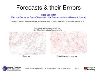
Forecasts & their Errrors Thanks to: Stefano Migliorini (NCEO), Mark Dixon (MetO), Mike Cullen (MetO), Roger Brugge (NCEO) Horiz. winds and pressure, at 5.5 km Met Office North Atlantic/European LAM Ross Bannister National Centre for Earth Observation (the Data Assimilation Research Centre) Forecast Possible error in forecast
Forecast errors • Forecast errors (from a numerical model): • are a fact of life! • depend upon the model formulation, • synoptic situation (‘flow dependent’), • model’s initial conditions, • length of the forecast. • are impossible to calculate in reality, δx = xf - xt. • Of interest: • forecast error statistics - the probability density fn. of xt, Pf(xt). • Applications: • probabilistic forecasting. • model evaluation/monitoring. • state estimation (data assimilation).
Seminar structure • Probability density functions (PDFs) of the state, Pf(xt). • The use of Pf(xt) in data assimilation problems. • Measuring Pf(xt). • Modelling Pf(xt) for large-scale data assimilation. • Refining Pf(xt) for large-scale data assimilation. • Challenges for small-scale Meteorology.
σ = √var(δx) PDF of state, Pf(xt) Forecast comprising a single number Pf(xt) xf = xt + δx 0 xt xf Probable state Impossible state Possible but unlikely state
σx2 = √var(δx2) σx1 = √var(δx1) cov(δx1,δx2) Two-component state vector Forecast comprising two numbers xf = xt + δx Pf(xt) 0
u –– v –– p –– T –– q xf = Geophysical error covariances – B • The B-matrix • specifies the PDF of errors in xf(Gaussianity assumed) • describes the uncertainty of each component of xf and • how errors of elements in xf are correlated • is important in data assimilation problems 107 – 108 elements δu δv δp δT δq B = δu δv δp δT δq 107 – 108 elements structure function associated (e.g.) with pressure at a location
Example standard deviations (square-root of variances) From Ingleby (2001)
Example geophysical structure functions (covariances with a fixed point) Univariate structure function Multivariate structure functions
t = 0 1.0 0.9 0.8 0.7 t > 0 1.0 0.9 0.8 0.7 Covariances are time dependent Structure function for tracer in simple transport model
Pf(xt) \ B in data assimilation • Data assimilation combines the PDFs of • forecast(s) from a dynamical model, Pf(xt)and • measurements, Pob(y|xt) • to allow an ‘optimal estimate’ to be found (Bayes’ Theorem). • Maximum likelihood solution (Gaussian PDFs) PDF of combination of forecast and observational information forecast = prior knowledge Solved e.g. by direct inversion or by variational methods
x(0) initial conditions y(t1) y(t2) y(t3) y(t4) y(t5) Tracer assimilation –– sources/ sinks Tracer + source/sink assimilation Data assimilation example(for inferred quantities) T, q, O3satellite radiances Initial conditionsinferred frommeasurements made at a later time Sources/sinks of tracer, rmeasurements of tracer r 30-day assimilation Pseudo satellite tracks
Dangers of misspecifying Pf(xt) \ B in data assimilation? Example 1: Anomalous correlations of moisture across an interface Example 2: Anomalous separability of structure functions around tilted structures Normally dry air Normally moist air
Measuring Pf(xt) \ B Forecast errors are impossible to measure in reality, δx = xf - xt. All proxy methods require a data assimilation system. Analysis of innovations Differences between varying length forecasts x √2 δx t Canadian ‘quick covs’ Ensembles x x √2 δx t t
PDF in model variables Transform to new variables that are assumed to be univariate 107 – 108 elements δu δv δp δT δq (multivariate) model variable (univariate) control variable control variable transform δu δv δp δT δq 107 – 108 elements Modelling Pf(xt) \ Bwith transforms for data assimilation
Ideas of ‘balance’ to formulate K (and hencePf(xt) \ B) these are not the same (clash of notation!) ← streamfunction (rot. wind) pert. (assume ‘balanced’) ← velocity potential (div. wind) pert. (assume ‘unbalanced’) ← residual pressure pert. (assume ‘unbalanced’) Implied f/c error covariance matrix H geostrophic balance operator (δψ → δpb) T hydrostatic balance operator (written in terms of temperature) Approach used at the ECMWF, Met Office, Meteo France, NCEP, MSC(SMC), HIRLAM, JMA, NCAR, CIRA Idea goes back to Parrish & Derber (1992)
Assumptions • This formulation makes many assumptions e.g.: • That forecast errors projected onto balanced variables are uncorrelated with those projected onto unbalanced variables. • The rotational wind is wholly a ‘balanced’ variable (i.e. large Bu regime). • That geostrophic and hydrostatic balances are appropriate for the motion being modelled (e.g. small Ro regime).
A. ‘Non-correlation’ test vertical model level latitude
Modified transform B. Rotational wind is not wholly balanced Could there be an unbalanced component of δψ? Standard transform H geostrophic balance operator T hydrostatic balance operator H anti-geostrophic balance operator
Modified transform Non-correlation test for refined model vertical model level latitude
from Berre, 2000 C. Are geostrophic and hydrostatic balances always appropriate? E.g. test for geostrophic balance
What next? Hi-resolution forecasts need hi-resolution Pf(xt) \ B • The Reading/MetO HRAA Collaboration • www.met.rdg.ac.uk/~hraa • Can forecast error covariances at hi-resolution be successfully modelled with the transform approach? • What is an appropriate transform at hi-resolution? • At what scales do hydrostatic and geostrophic balance become inappropriate? • There is little known theory to guide us at hi-res. • → What is the structure of forecast error covariances in such cases? High impact weather!
Hi-resolution ensembles Early results from Met Office 1.5 km LAM (a MOGREPS-like system) Thanks to Mark Dixon (MetO), Stefano Migliorini (NCEO), Roger Brugge (NCEO)
Summary • All measurements are inaccurate and all forecasts are wrong! • Accurate knowledge of forecast uncertainty (PDF) is useful: » to allow range of possible outcomes to be predicted, » to give allowed ways that a forecast can be modified by observations (data assimilation). • For synoptic/large scales the forecast error PDF is modelled with a change of variables and balance relations. • For hi-res (convective scales) the forecast error PDF is still important but there is no formal theory to guide PDF modelling: » hydrostatic/geostrophic balance less appropriate, » non-linearity/dynamic tendencies may be more important.