Download
1 / 31
380 likes | 696 Views
Erik de Jong & Willem Bouma. Octree-based Point-Cloud Compression. Introduction. Arithmetic Coding Octree Compression Surface Approximation Child Cells Configurations Single Child cell configurations Results Questions. Arithmetic Coding.

E N D
Erik de Jong & Willem Bouma Octree-basedPoint-CloudCompression
Introduction • Arithmetic Coding • Octree • Compression • Surface Approximation • Child Cells Configurations • Single Child cell configurations • Results • Questions
Arithmetic Coding • Assign to every symbol a range from the interval [0-1]. The size of the range represents the probability of the symbol occurring. Example: A: 60% [ 0.0, 0.6 ) B: 20% [ 0.6, 0.8 ) C: 10% [ 0.8, 0.9 ) D: 10% [ 0.9, 1.0 ) (end of data symbol)
Arithmetic Coding A B C D Ranges: A – [0,0.6), B – [0.6,0.8), C – [0.8,0.9), D – [0.9,1) The example shows the decoding of 0.538.
Huffman • Huffman coding is a specialized case of arithmetic coding • Every symbol is converted to a bit sequence of integer length • Probabilities are rounded to negative powers of two • Advantage: Can decode parts of the input stream • Disadvantage: Arithmetic coding comes much closer to the optimal entropy encoding
Context SQUEEL
Compression • Estimate/Approximate as much as possible • Store only the differences w.r.t. the estimate • A better estimate -> • smaller numbers • lower entropy • better compression
Octree • What is an Octree?
Octree • Per cell we store only the occupied child cells • Options: • Store a single byte, each bit representing a child cell (for example 11001100) • Store the number of occupied cells eand a tupel T with the indices of the occupied cells (for example e=4, T={0,1,4,5})
Compression • We willapproximate/estimate/compress: • The surface • Number of non-emptychildcells • Childcellconfiguration • Index compression • Single childcellconfiguration
SurfaceApproximation • Every level of the octree will yield a preliminary approximation Q of the complete point cloud P • For a cell that is to be subdivided: • Predict surface F based on Moving Least Squares (MLS) on k nearest points in Q
Number of non-emptycells • Prediction of number of non-empty cells e • Based on estimation of the sampling density ρ • Local sampling density ρiat point piin P: • k, nearest points • pi, point in the point cloud P • qi, point on the surface approximation Q
Number of non-emptycells • Sampling density: • Guess the number of child cells e based on: • The area of the plane F • The sampling density ρ
Number of non-emptycells • Quality of prediction • Graphs show the difference between te estimated value and the true value. • The level 5 octree • The level 7 octree • The entire octree.
Childcellconfiguration • Given the number of non-empty child cells e there are only a limited number of configurations:
Childcellconfiguration • We have an array with all weighted possible configurations, sorted in ascending order • Each configuration of the subdivision is encoded as an index of the array. • Common configurations get lower weights, means smaller indices, means lower entropy.
Childcellconfiguration • Cell centers tend to be close to F.
Childcellconfiguration • To find the weight of a configuration: • Sum up the (L1) distances from the cell centers to F
Index Compression • Index of the configuration in the sorted array is encoded using arithmetic coding under two contexts • First context: the octree level of the cell C • Second context: the expressiveness e(F)
Index Compression • e(F) reflects the angle of the plane to the coordinate directions
Index Compression • In order to use e(F) as a context for arithmetic coding it has to be quantized. • It has been found that five bins was sufficient and delivered the best results.
Single childcellconfiguration • We can exploit an observation for cells that have only one occupied child cell. • Scanning devices often have a regular sampling grid. • It is possible to predict samples on the surface, rather than just close to the surface. • This is relevant for the finer levels in the octree hierarchy.
Single child cell configuration • For cells with only one child cell we can predict T based on the nearest neighbours of points m, centroid of the k nearest neighbours
Single childcellconfiguration • Quite suprisingly, the cell center projections on F that are farthest away are most likely to be occupied. • The area farther away can be seen as undersampled. • So a sample in that area becomes more likely since we expect the surface to be regular and no undersampling should exist.
Single childcellconfiguration • The weights for the eight possible configurations are given as c(T), cell center of T prj(F,c(T)), projection of c(T) on F
Otherattributes • Extra attributes can be encoded with an octree • Color • Normals
Otherattributes • Compressing color • Same two-step method as with coordinates • Different prediction functions are needed
Results (bpp) Bits Per Point Rawsize is assumed to use 3 times 4 Bytes per point. The octreeuses 12 levels. Exceptforthe Dragon forwhichit is unknown.
Results (b) uses 1.89 bpp