Download
1 / 63
630 likes | 801 Views
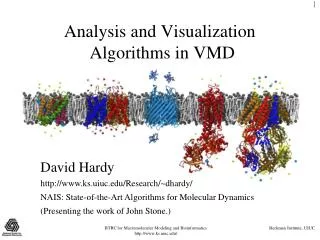
GPU Accelerated Visualization and Analysis in VMD and Recent NAMD Developments. John Stone Theoretical and Computational Biophysics Group Beckman Institute for Advanced Science and Technology University of Illinois at Urbana-Champaign http://www.ks.uiuc.edu/Research/gpu/

E N D
GPU Accelerated Visualization and Analysis in VMDandRecent NAMD Developments John Stone Theoretical and Computational Biophysics Group Beckman Institute for Advanced Science and Technology University of Illinois at Urbana-Champaign http://www.ks.uiuc.edu/Research/gpu/ GPU Technology Conference Fairmont Hotel, San Jose, CA, October 1, 2009
VMD – “Visual Molecular Dynamics” • Visualization and analysis of molecular dynamics simulations, sequence data, volumetric data, quantum chemistry simulations, particle systems, … • User extensible with scripting and plugins • http://www.ks.uiuc.edu/Research/vmd/
Range of VMD Usage Scenarios • Users run VMD on a diverse range of hardware: laptops, desktops, clusters, and supercomputers • Typically used as a desktop application, for interactive 3D molecular graphics and analysis • Can also be run in pure text mode for numerically intensive analysis tasks, batch mode movie rendering, etc… • GPU acceleration provides an opportunity to make some slow, or batch calculations capable of being run interactively, or on-demand…
Need for Multi-GPU Acceleration in VMD • Ongoing increases in supercomputing resources at NSF centers such as NCSA enable increased simulation complexity, fidelity, and longer time scales… • Drives need for more visualization and analysis capability at the desktop and on clusters running batch analysis jobs • Desktop use is the most compute-resource-limited scenario, where GPUs can make a big impact…
CUDA Acceleration in VMD Electrostatic field calculation, ion placement 20x to 44x faster Molecular orbital calculation and display 100x to 120x faster Imaging of gas migration pathways in proteins with implicit ligand sampling 20x to 30x faster
Electrostatic Potential Maps • Electrostatic potentials evaluated on 3-D lattice: • Applications include: • Ion placement for structure building • Time-averaged potentials for simulation • Visualization and analysis Isoleucine tRNA synthetase
Infinite vs. Cutoff Potentials • Infinite range potential: • All atoms contribute to all lattice points • Quadratic time complexity • Cutoff (range-limited) potential: • Atoms contribute within cutoff distance to lattice points resulting in linear time complexity • Used for fast decaying interactions (e.g. Lennard-Jones, Buckingham) • Fast full electrostatics: • Replace electrostatic potential with shifted form • Combine short-range part with long-range approximation • Multilevel summation method (MSM), linear time complexity
Short-range Cutoff Summation • Each lattice point accumulates electrostatic potential contribution from atoms within cutoff distance: if (rij < cutoff) potential[j] += (charge[i] / rij) * s(rij) • Smoothing function s(r) is algorithm dependent Cutoff radius rij: distance from lattice[j] to atom[i] Lattice point j being evaluated atom[i]
Cutoff Summation on the GPU Atoms are spatially hashed into fixed-size bins CPU handles overflowed bins (GPU kernel can be very aggressive) GPU thread block calculates corresponding region of potential map, Bin/region neighbor checks costly; solved with universal table look-up Each thread block cooperatively loads atom bins from surrounding neighborhood into shared memory for evaluation Shared memory atom bin Global memory Constant memory Offsets for bin neighborhood Potential map regions Look-up table encodes “logic” of spatial geometry Bins of atoms
GPU cutoff with CPU overlap: 17x-21x faster than CPU core If asynchronous stream blocks due to queue filling, performance will degrade from peak… Cutoff Summation Performance GPU acceleration of cutoff pair potentials for molecular modeling applications. C. Rodrigues, D. Hardy, J. Stone, K. Schulten, W. Hwu. Proceedings of the 2008 Conference On Computing Frontiers, pp. 273-282, 2008.
Cutoff Summation Observations • Use of CPU to handle overflowed bins is very effective, overlaps completely with GPU work • Caveat: Overfilling stream queue can trigger blocking behavior. Recent drivers queue >100 ops before blocking. • Higher precision: • Compensated summation (all GPUs) or double-precision (GT200 only) only a ~10% performance penalty vs. single-precision arithmetic • Next-gen “Fermi” GPUs will have an even lower performance cost for double-precision arithmetic
Multilevel Summation Method • Approximates full electrostatic potential • Calculates sum of smoothed pairwise potentials interpolated from a hierarchy of lattices • Advantages over particle-mesh Ewald, fast multipole: • Algorithm has linear time complexity • Permits non-periodic and periodic boundaries • Produces continuous forces for dynamics (advantage over FMM) • Avoids 3-D FFTs for better parallel scaling (advantage over PME) • Spatial separation allows use of multiple time steps • Can be extended to other pairwise interactions • Skeel, Tezcan, Hardy, J Comp Chem, 2002 — Computing forces for molecular dynamics • Hardy, Stone, Schulten, J Paral Comp, 2009 — GPU-acceleration of potential map calculation
Multilevel Summation Main Ideas • Split the 1/r potential into a short-range cutoff part plus smoothed parts that are successively more slowly varying. All but the top level potential are cut off. • Smoothed potentials are interpolated from successively coarser lattices. • Finest lattice spacing h and smallest cutoff distance a are doubled at each successive level. Split the 1/r potential Interpolate the smoothed potentials 2h-lattice + 1/r = h-lattice + atoms a 2a
Multilevel Summation Calculation exact short-range interactions interpolated long-range interactions map potential Computational Steps 4h-lattice long-range parts prolongation restriction 2h-lattice cutoff prolongation restriction h-lattice cutoff anterpolation interpolation atom charges short-range cutoff map potentials
Cutoff radius Sphere of lattice point charges Accumulate potential Lattice Cutoff Summation • Each lattice point accumulates electrostatic potential contribution from all lattice point charges within cutoff distance • Relative distances are the same between points on a uniform lattice, multiplication by a precomputed stencil of “weights” • Weights at each level are identical up to a scaling factor (due to choice of splitting and doubling of lattice spacing and cutoff) • Calculate as 3D convolution of sub-cube of lattice point charges with enclosing cube of weights
Each thread block cooperatively loads lattice charge regions into shared memory for evaluation, multiply by weight stencil from constant memory Shared memory Sub-regions of lattice charge Constant memory Global memory Lattice potential regions Lattice charge regions Stencil of weights Lattice Cutoff Summation on GPU • Store stencil of weights in constant memory • Thread blocks calculate 4x4x4 regions of lattice potentials • Load nearby regions of lattice charges into shared memory • Evaluate all lattice levels concurrently, scaling by level factor (keeps GPU from running out of work at upper lattice levels)
Evaluation Using Sliding Window • Every thread in block needs to simultaneously read and use the same weight from constant memory • Read 8x8x8 block (8 regions) of lattice charges into shared memory • Slide 4x4x4 window by 4 shifts along each dimension
Multilevel Summation on the GPU Accelerate short-range cutoff and lattice cutoff parts Performance profile for 0.5 Å map of potential for 1.5 M atoms. Hardware platform is Intel QX6700 CPU and NVIDIA GTX 280.
Photobiology of Vision and Photosynthesis Investigations of the chromatophore, a photosynthetic organelle Light Partial model: ~10M atoms Electrostatics needed to build full structural model, place ions, study macroscopic properties Electrostatic field of chromatophore model from multilevel summation method: computed with 3 GPUs (G80) in ~90 seconds, 46x faster than single CPU core Full chromatophore model will permit structural, chemical and kinetic investigations at a structural systems biology level
Computing Molecular Orbitals • Visualization of MOs aids in understanding the chemistry of molecular system • MO spatial distribution is correlated with probability density for an electron(s) • Calculation of high resolution MO grids can require tens to hundreds of seconds on CPUs
Animating Molecular Orbitals • Animation of (classical mechanics) molecular dynamics trajectories provides insight into simulation results • To do the same for QM or QM/MM simulations one must compute MOs at ~10 FPS or more • >100x speedup (GPU) over existing tools now makes this possible! C60
Molecular Orbital Computation and Display Process One-time initialization Read QM simulation log file, trajectory Initialize Pool of GPU Worker Threads Preprocess MO coefficient data eliminate duplicates, sort by type, etc… For current frame and MO index, retrieve MO wavefunction coefficients Compute 3-D grid of MO wavefunction amplitudes Most performance-demanding step, run on GPU… For each trj frame, for each MO shown Extract isosurface mesh from 3-D MO grid Apply user coloring/texturing and render the resulting surface
CUDA Block/Grid Decomposition MO 3-D lattice decomposes into 2-D slices (CUDA grids) Grid of thread blocks: 0,0 0,1 … 1,0 1,1 … Small 8x8 thread blocks afford large per-thread register count, shared mem. Threads compute one MO lattice point each. … … … Padding optimizes glob. mem perf, guaranteeing coalescing
MO Kernel for One Grid Point (Naive C) Loop over atoms … for (at=0; at<numatoms; at++) { int prim_counter = atom_basis[at]; calc_distances_to_atom(&atompos[at], &xdist, &ydist, &zdist, &dist2, &xdiv); for (contracted_gto=0.0f, shell=0; shell < num_shells_per_atom[at]; shell++) { int shell_type = shell_symmetry[shell_counter]; for (prim=0; prim < num_prim_per_shell[shell_counter]; prim++) { float exponent = basis_array[prim_counter ]; float contract_coeff = basis_array[prim_counter + 1]; contracted_gto += contract_coeff * expf(-exponent*dist2); prim_counter += 2; } for (tmpshell=0.0f, j=0, zdp=1.0f; j<=shell_type; j++, zdp*=zdist) { int imax = shell_type - j; for (i=0, ydp=1.0f, xdp=pow(xdist, imax); i<=imax; i++, ydp*=ydist, xdp*=xdiv) tmpshell += wave_f[ifunc++] * xdp * ydp * zdp; } value += tmpshell * contracted_gto; shell_counter++; } } ….. Loop over shells Loop over primitives: largest component of runtime, due to expf() Loop over angular momenta (unrolled in real code)
MO GPU Kernel Snippet:Contracted GTO Loop, Use of Constant Memory [… outer loop over atoms …] float dist2 = xdist2 + ydist2 + zdist2; // Loop over the shells belonging to this atom (or basis function) for (shell=0; shell < maxshell; shell++) { float contracted_gto = 0.0f; // Loop over the Gaussian primitives of this contracted basis function to build the atomic orbital int maxprim = const_num_prim_per_shell[shell_counter]; int shelltype = const_shell_types[shell_counter]; for (prim=0; prim < maxprim; prim++) { float exponent = const_basis_array[prim_counter ]; float contract_coeff = const_basis_array[prim_counter + 1]; contracted_gto += contract_coeff * __expf(-exponent*dist2); prim_counter += 2; } [… continue on to angular momenta loop …] Constant memory: nearly register-speed when array elements accessed in unison by all peer threads….
MO GPU Kernel Snippet:Unrolled Angular Momenta Loop Loop unrolling: • Saves registers (important for GPUs!) • Reduces loop control overhead • Increases arithmetic intensity /* multiply with the appropriate wavefunction coefficient */ float tmpshell=0; switch (shelltype) { case S_SHELL: value += const_wave_f[ifunc++] * contracted_gto; break; [… P_SHELL case …] case D_SHELL: tmpshell += const_wave_f[ifunc++] * xdist2; tmpshell += const_wave_f[ifunc++] * xdist * ydist; tmpshell += const_wave_f[ifunc++] * ydist2; tmpshell += const_wave_f[ifunc++] * xdist * zdist; tmpshell += const_wave_f[ifunc++] * ydist * zdist; tmpshell += const_wave_f[ifunc++] * zdist2; value += tmpshell * contracted_gto; break; [... Other cases: F_SHELL, G_SHELL, etc …] } // end switch
Preprocessing of Atoms, Basis Set, and Wavefunction Coefficients • Must make effective use of high bandwidth, low-latency GPU on-chip memory, or CPU cache: • Overall storage requirement reduced by eliminating duplicate basis set coefficients • Sorting atoms by element type allows re-use of basis set coefficients for subsequent atoms of identical type • Padding, alignment of arrays guarantees coalesced GPU global memory accesses, CPU SSE loads
GPU Traversal of Atom Type, Basis Set, Shell Type, and Wavefunction Coefficients Monotonically increasing memory references Constant for all MOs, all timesteps • Loop iterations always access same or consecutive array elements for all threads in a thread block: • Yields good constant memory cache performance • Increases shared memory tile reuse Different at each timestep, and for each MO Strictly sequential memory references
Use of GPU On-chip Memory • If total data less than 64 kB, use only const mem: • Broadcasts data to all threads, no global memory accesses! • For large data, shared memory used as a program-managed cache, coefficients loaded on-demand: • Tiles sized large enough to service entire inner loop runs, broadcast to all 64 threads in a block • Complications: nested loops, multiple arrays, varying length • Key to performance is to locate tile loading checks outside of the two performance-critical inner loops • Only 27% slower than hardware caching provided by constant memory (GT200) • Next-gen “Fermi” GPUs will provide larger on-chip shared memory, L1/L2 caches, reduced control overhead
Array tile loaded in GPU shared memory. Tile size is a power-of-two, multiple of coalescing size, and allows simple indexing in inner loops (array indices are merely offset for reference within loaded tile). Surrounding data, unreferenced by next batch of loop iterations 64-Byte memory coalescing block boundaries Full tile padding Coefficient array in GPU global memory
MO GPU Kernel Snippet:Loading Tiles Into Shared Memory On-Demand [… outer loop over atoms …] if ((prim_counter + (maxprim<<1)) >= SHAREDSIZE) { prim_counter += sblock_prim_counter; sblock_prim_counter = prim_counter & MEMCOAMASK; s_basis_array[sidx ] = basis_array[sblock_prim_counter + sidx ]; s_basis_array[sidx + 64] = basis_array[sblock_prim_counter + sidx + 64]; s_basis_array[sidx + 128] = basis_array[sblock_prim_counter + sidx + 128]; s_basis_array[sidx + 192] = basis_array[sblock_prim_counter + sidx + 192]; prim_counter -= sblock_prim_counter; __syncthreads(); } for (prim=0; prim < maxprim; prim++) { float exponent = s_basis_array[prim_counter ]; float contract_coeff = s_basis_array[prim_counter + 1]; contracted_gto += contract_coeff * __expf(-exponent*dist2); prim_counter += 2; } [… continue on to angular momenta loop …]
VMD MO Performance Results for C60Sun Ultra 24: Intel Q6600, NVIDIA GTX 280 C60 basis set 6-31Gd. We used an unusually-high resolution MO grid for accurate timings. A more typical calculation has 1/8th the grid points. * Runtime-generated JIT kernel compiled using batch mode CUDA tools **Reduced-accuracy approximation of expf(), cannot be used for zero-valued MO isosurfaces
Performance Evaluation:Molekel, MacMolPlt, and VMD Sun Ultra 24: Intel Q6600, NVIDIA GTX 280
VMD Orbital Dynamics Proof of Concept One GPU can compute and animate this movie on-the-fly! CUDA const-cache kernel, Sun Ultra 24, GeForce GTX 285 threonine With GPU speedups over 100x, previously insignificant CPU surface gen, gradient calc, and rendering are now 66% of runtime. Need GPU-accelerated surface gen next…
Multi-GPU Load Balance • Many early CUDA codes assumed all GPUs were identical • All new NVIDIA cards support CUDA, so a typical machine may have a diversity of GPUs of varying capability • Static decomposition works poorly for non-uniform workload, or diverse GPUs, e.g. w/ 2 SM, 16 SM, 30 SM GPU 1 2 SMs GPU 3 30 SMs …
Multi-GPU Dynamic Work Distribution Dynamic work distribution // Each GPU worker thread loops over // subset 2-D planes in a 3-D cube… while (!threadpool_next_tile(&parms, tilesize, &tile){ // Process one plane of work… // Launch one CUDA kernel for each // loop iteration taken… // Shared iterator automatically // balances load on GPUs } GPU 1 GPU 3 …
Multi-GPU Runtime Error/Exception Handling • Competition for resources from other applications or the windowing system can cause runtime failures (e.g. GPU out of memory half way through an algorithm) • Handling of algorithm exceptions (e.g. convergence failure, NaN result, etc) • Need to handle and/or reschedule failed tiles of work GPU 1 SM 1.0 128MB GPU 3 SM 1.3 4096MB …
Some Example Multi-GPU Latencies Relevant to Interactive Sci-Viz Apps 8.4us CUDA empty kernel (immediate return) 10.0us Sleeping barrier primitive (non-spinning barrier that uses POSIX condition variables to prevent idle CPU consumption while workers wait at the barrier) 20.3us pool wake / exec / sleep cycle (no CUDA) 21.4us pool wake / 1 x (tile fetch) / sleep cycle (no CUDA) 30.0us pool wake / 1 x (tile fetch / CUDA nop kernel) / sleep cycle, test CUDA kernel computes an output address from its thread index, but does no output 1441.0us pool wake / 100 x (tile fetch / CUDA nop kernel) / sleep cycle test CUDA kernel computes an output address from its thread index, but does no output
VMD Multi-GPU Molecular Orbital Performance Results for C60 Intel Q6600 CPU, 4x Tesla C1060 GPUs, Uses persistent thread pool to avoid GPU init overhead, dynamic scheduler distributes work to GPUs
VMD Multi-GPU Molecular Orbital Performance Results for C60Using Mapped Host Memory Intel Q6600 CPU, 3x Tesla C1060 GPUs, GPU kernel writes output directly to host memory, no extra cudaMemcpy() calls to fetch results! See cudaHostAlloc() + cudaGetDevicePointer()
MO Kernel Structure, Opportunity for JIT…Data-driven, but representative loop trip counts in (…) Loop over atoms (1 to ~200) { Loop over electron shells for this atom type (1 to ~6) { Loop over primitive functions for this shell type (1 to ~6) { } Unpredictable (at compile-time, since data-driven ) but small loop trip counts result in significant loop overhead. Dynamic kernel generation and JIT compilation can unroll entirely, resulting in 40% speed boost Loop over angular momenta for this shell type (1 to ~15) {} } }
Molecular Orbital Computation and Display ProcessDynamic Kernel Generation, Just-In-Time (JIT) C0mpilation Read QM simulation log file, trajectory One-time initialization Preprocess MO coefficient data eliminate duplicates, sort by type, etc… Initialize Pool of GPU Worker Threads Generate/compile basis set-specific CUDA kernel For current frame and MO index, retrieve MO wavefunction coefficients Compute 3-D grid of MO wavefunction amplitudes using basis set-specific CUDA kernel For each trj frame, for each MO shown Extract isosurface mesh from 3-D MO grid Render the resulting surface
….. // loop over the shells belonging to this atom (or basis function) for (shell=0; shell < maxshell; shell++) { float contracted_gto = 0.0f; // Loop over the Gaussian primitives of this contracted // basis function to build the atomic orbital int maxprim = const_num_prim_per_shell[shell_counter]; int shell_type = const_shell_symmetry[shell_counter]; for (prim=0; prim < maxprim; prim++) { float exponent = const_basis_array[prim_counter ]; float contract_coeff = const_basis_array[prim_counter + 1]; contracted_gto += contract_coeff * exp2f(-exponent*dist2); prim_counter += 2; } /* multiply with the appropriate wavefunction coefficient */ float tmpshell=0; switch (shell_type) { case S_SHELL: value += const_wave_f[ifunc++] * contracted_gto; break; […..] case D_SHELL: tmpshell += const_wave_f[ifunc++] * xdist2; tmpshell += const_wave_f[ifunc++] * ydist2; tmpshell += const_wave_f[ifunc++] * zdist2; tmpshell += const_wave_f[ifunc++] * xdist * ydist; tmpshell += const_wave_f[ifunc++] * xdist * zdist; tmpshell += const_wave_f[ifunc++] * ydist * zdist; value += tmpshell * contracted_gto; break; ….. contracted_gto = 1.832937 * expf(-7.868272*dist2); contracted_gto += 1.405380 * expf(-1.881289*dist2); contracted_gto += 0.701383 * expf(-0.544249*dist2); // P_SHELL tmpshell = const_wave_f[ifunc++] * xdist; tmpshell += const_wave_f[ifunc++] * ydist; tmpshell += const_wave_f[ifunc++] * zdist; value += tmpshell * contracted_gto; contracted_gto = 0.187618 * expf(-0.168714*dist2); // S_SHELL value += const_wave_f[ifunc++] * contracted_gto; contracted_gto = 0.217969 * expf(-0.168714*dist2); // P_SHELL tmpshell = const_wave_f[ifunc++] * xdist; tmpshell += const_wave_f[ifunc++] * ydist; tmpshell += const_wave_f[ifunc++] * zdist; value += tmpshell * contracted_gto; contracted_gto = 3.858403 * expf(-0.800000*dist2); // D_SHELL tmpshell = const_wave_f[ifunc++] * xdist2; tmpshell += const_wave_f[ifunc++] * ydist2; tmpshell += const_wave_f[ifunc++] * zdist2; tmpshell += const_wave_f[ifunc++] * xdist * ydist; tmpshell += const_wave_f[ifunc++] * xdist * zdist; tmpshell += const_wave_f[ifunc++] * ydist * zdist; value += tmpshell * contracted_gto; General loop-based CUDA kernel Dynamically-generated CUDA kernel (JIT)
NAMD: Molecular Dynamics on GPUs http://www.ks.uiuc.edu/Research/gpu/ http://www.ks.uiuc.edu/Research/namd/
Biomolecular Time Scales Max Timestep: 1 fs
Typical Simulation Statistics • 100,000 atoms (including water, lipid) • 10-20 MB of data for entire system • 100 Å per side periodic cell • 12 Å cutoff of short-range nonbonded terms • 10,000,000 timesteps (10 ns) • 3 s/step on one processor (1 year total!)
NAMD Hybrid Parallel Decomposition Kale et al.,J. Comp. Phys.151:283-312, 1999. • Spatially decompose data and communication. • Separate but related work decomposition. • “Compute objects” facilitate iterative, measurement-based load balancing system.
NAMD Parallel Molecular Dynamics: Overlapping CPU/GPU Execution Example Configuration 108 847 objects 100,000 Offload to GPU Objects are assigned to processors and queued as data arrives. Phillips et al., SC2002. Phillips et al., SC2008.
Overlapping GPU/CPU Computation with Communication GPU Remote Force f Local Force f x x CPU Remote Local f Local Update x f x Other Nodes/Processes One Timestep: want total runtime < 1ms
Nonbonded Forces on CUDA GPU • Most expensive calculation (~95% runtime in CPU versions) • Work decomposed into patch pairs, as in regular NAMD Force computation on single multiprocessor 16kB Shared Memory Patch A Coordinates & Parameters Texture Unit Force Table Interpolation Thread block w/ 64 threads Constants Exclusions 32kB Registers Patch B Coords, Params, & Forces 8kB cache 8kB cache Main Memory, hundreds of cycles of latency Stone et al., J. Comp. Chem. 28:2618-2640, 2007.