Dr Ben Matthews ben@chooseclimate (mobile)+32 472 987028 (ring me to arrange a demonstration)

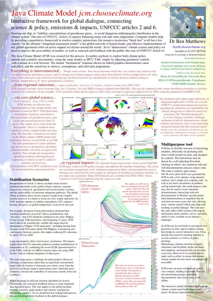
1. Java Climate Model jcm.chooseclimate.org Interactive framework for global dialogue, connecting science & policy, emissions & impacts, UNFCCC articles 2 and 6. Steering our ship, to “stabilise concentrations of greenhouse gases... to avoid dangerous anthropogenic interference in the climate system” (the aim of UNFCCC, Article 2) requires balancing many risk and value judgements. Computer models help by providing a quantitative framework to resolve complex interactions, but remain a mysterious “black box” to all but a few experts. Yet the ultimate “integrated assessment model” is the global network of human heads, and effective implementation of any global agreement relies on active support of citizens around the world. So to “democratise” climate science and policy we need to improve the accessibility of models, as well as outreach and feedback with the public (the task of UNFCCC Article 6). The author, responding to changing weather to steer to a “safe landing”? Dr Ben Matthews ben@chooseclimate.org (mobile)+32 472 987028 (ring me to arrange a demonstration) Currently based at: Institut d'Astronomie et de Géophysique, Université Catholique de Louvain, Belgium (working with Prof Jean-Pascal vanYpersele) JCM was also developed with: Klima & UmweltPhysik, University Bern DEA-CCAT/Energimiljoradet, Copenhagen UNEP-GRID Arendal, Norway The Java Climate Model (JCM) was created for this process. It enables anybody to explore both climate policy options and scientific uncertainties, using the same models as IPCC-TAR, simply by adjusting parameter controls with a mouse in a web browser. The instant “mechanical” response shown on linked graphics demonstrates cause and effect, and the sensitivity to choices, assumptions, and risk/value judgements. Everything is interconnected... People want to know how local emissions which they can control, may influence the vast global natural and human systems, and so change local climate impacts which affect them directly. In the example below, the main cause-effect chain goes anti-clockwise from the top, but total emissions are calculated by an inverse iteration method aiming to stabilise temperature at 2C above preindustrial (as below). ...from regional emissions... (upper-right plots, curves for 12 regions, colours as map, from 1900-2100)JCM currently includes socio-economic data for 12 regions, for each SRES scenario (adapted from IMAGE). This may be combined with various distribution formulae to calculate regional CO2 emissions. In the example, CO2 emissions follow Kyoto targets to 2012, then converge to equal per-capita levels by 2050, using the population fromSRES A1B. ...via core global science... (lower-left plots , from 1750 to 2300). JCM includes an efficient java implementation of the simple models and formulae as used for IPCC-TAR projections. Atmospheric chemistry and radiative forcing includes all greenhouse gases, plus ozone and aerosol precursors (total 35 gases). The carbon cycle comes from the Bern model. There is a feedback from climate to carbon, coupled within one time-loop. The heat flux calculations are based on the Wigley-Raper UDEB model with parameters fitted to seven GCMs as in TAR. The slow penetration of carbon and heat into the oceans is calculated by upwelling-diffusion models solved by an eigenvector method. This includes the temperature-upwelling feedback affecting thermal expansion, to which ice-melt is added to calculate sea-level rise. Correspondence with IPCC predictions may be demonstrated by superimposed data. The attribution plot (upper right) illustrates an integrated application of JCM, for a recent UNFCCC model intercomparison exercise regarding the attribution of responsibility for climate change due to different sources of emissions (the “Brazilian proposal”). As well as being a scientific challenge, attribution of effects from processes which combine non-linearly raises some interesting intergenerational and inter-regional equity issues. (note, the attribution calculations are not yet adapted for stabilisation scenarios, so this plot is not consistent with others in this example) Multipurpose tool JCM has an flexible structure of interacting modules, efficiently recalculating only what is both needed for plots and changed by controls. The interactions may be shown by a self-adjusting flowchart, clicking on which also summons relevant web documentation and java source code. The code is entirely open source. The 98-curve plots (left) were generated by JCM in only a few minutes, using internet explorer, and a simple text scripting code. As well as for batch calculations in problem-solving frameworks, this multi-purpose code may also be used to create automatic demonstrations, interacting with web documentation to illustrate specific points. Such demonstrations or snapshots may be sent between users across the web, allowing some “remote control”which may help with teaching or global dialogue. The code uses the same object-label system as the pop-up information about controls, curves, and units, which is now available in ten (human!) languages. So JCM may be used both to investigate new questions (as left), and to explain existing knowledge in a novel interactive way. It has already been used for teaching students in several countries, as well as at policy meetings. Maintaining a balance between scientific robustness and flexibility on the one hand, and simplicity and interactivity on the other, is not easy. However it is essential that we make such an effort, to ensure that serious climate models become more transparent and accessible. JCM works on most web browsers and is very compact, loading in seconds. You can also download packages, including documentation and source code, to use offline. The interactive model illustrates itself and the climate system much better than a static poster. So please experiment for yourself! ...to regional impacts The regional climate map (centre) shows recent HadCM3 GCM data, scaled to JCM global average, and added to the baseline climatology. The colors mix maximum-temperature (red), minimum temperature (blue), and preciptitation (green). Averages are calculated for each country or subregion. Everything recalculates instantly, as you adjust any parameter. Many GCM datasets are available from IPCC-DDC, whose visualiser is now being updated using the same java code. Stabilisation Scenarios Interpretation of Article 2 (above) includes many factors: nonlinear thresholds in theglobal climate response, regional impacts on ecological, agricultural and socioeconomic systems, and the achievability of emissions mitigation pathways. The global debate to balance these factors requires insight from complex models, however it is likely to focus on a few simple indicators. So JCM includes options to stabilise atmospheric CO2, radiative forcing (all gases), or global temperature, at any level and year. For example, European Union policymakers proposed that warming should not exceed 2C (above preindustrial), and “therefore”, that CO2 should be stabilised at less than 550ppm. Using average TAR parameters, and mitigating 21 gases, JCM shows that to be scientifically credible this target must be interpreted as 550ppm “CO2 equivalent”, including forcing from all gases (with CO2 alone about 450-500ppm). Considering also convergence between regions, this implies reducing EU emissions by about 75% by 2050. Large uncertainties affect such inverse calculations. The figures (right) show 98 CO2 emissions pathways leading tostabilisation of temperature at 2C, combining the seven GCMs (parameterised as in the TAR), with the six SRES scenarios (plus one using 2000 levels), with an without mitigation of other gases. The wide range poses a challenge for policymakers! However, selecting a temperature rather than an equivalent concentration target shifts the burden of managing uncertainty away from the receivers of climate impacts (particularly more vulnerable poor countries), towards the controllers of emissions (mostly from rich countries). When designing an efficient iteration algorithm for inverse calculations, the correction-feedback process is more important than the initial guess. This also applies to the global iteration between scientists, policymakers and citizens, essential for interpreting Article 2. So we should not fear making bold guesses, but need to design better feedback in the global dialogue. The redder set of 49 curves have no mitigation of non-CO2 gases, whilst the other 49 assume that emissions of each gas (including aerosol and ozone precursors) are reduced by an equal proportion, compared to the SRES baseline in each year. CO2 Emissions (fossil + landuse) GtC/yr Global Average Temperature The same stes of curves as above. The greener curves correspond to cooler GCMs. The baseline is preindustrial, hence there is already divergence at 2000. For a few scenarios (hottest model GFDL + large other gas emissions in SRESA2) the iteration failed to find a pathway below 2C