Escaping Local Optima

1. Escaping Local Optima

2. Where are we? Optimization methods Complete solutions Partial solutions Exhaustive search Branch and bound Greedy Best first A* Divide and Conquer Dynamic programming Constraint Propagation Exhaustive search Hill climbing Random restart General Model of Stochastic Local Search Simulated Annealing Tabu search

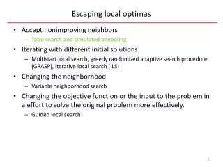
3. Escaping local optima Stochastic local search • many important algorithms address the problem of avoiding the trap of local optima (possible source of project topics) • Michalewicz & Fogel focus on two only • simulated annealing • tabu search

4. Formal model of Stochastic Local Search (SLS): Hoos and Stützle goal: abstract the simple search subroutines from high level control structure experiment with various search methods systematically

5. Formal model of Stochastic Local Search (SLS): Hoos and Stützle Generalized Local Search Machine (GLSM) M M =(Z, z0, M, m0, Δ, σZ, σΔ, ΤZ, ΤΔ) Z: set of states (basic search strategies) z0 ∈ Z : start state M: memory space m0 ∈ M : start memory state Δ ⊆ Z×Z : transition relation (when to switch to another type of search) σZ : set of state types; σΔ : set of transition types ΤZ : Z ➝ σZ associate states with types ΤΔ : Δ ➝ σΔ associate transitions with types

6. (0) Basic Hill climbing determine initial solution s while s not local optimum choose s’ in N(s) such that f(s’)>f(s) s = s’ return s Det Det z0 z1 M =(Z, z0, M, m0, Δ, σZ, σΔ, ΤZ, ΤΔ) Z: {z0, z1} M: {m0} //not used in this model Δ ⊆ Z×Z :{ (zo, z1), (z1, z1)} σZ : { random choice, select better neighbour } σΔ : { Det} ΤZ : ΤZ (z0) = random choice, ΤZ(z1) = select better neighbour ΤΔ : ΤΔ ((zo, z1)) = Det,ΤΔ((z1, z1)) = Det

7. (1) Randomized Hill climbing determine initial solution s; bestS = s while termination condition not satisfied with probability p choose neighbour s’ at random else //climb if possible choose s’ with f(s’) > f(s) s = s’; if (f(s) > f(bestS)) bestS = s return bestS

8. (1) Randomized Hill climbing M =(Z, z0, M, m0, Δ, σZ, σΔ, ΤZ, ΤΔ) • Z: {z0, z1, z2} M: {m0} • Δ ⊆ Z×Z :{(zo, z1),(z1, z1),(zo, z2),(z1, z2),(z2, z1),(z2, z2)} • σZ : { random choice, select better neighbour, select any neighbour } σΔ : { Prob(p), Prob(1-p)} • ΤZ : ΤZ (z0) = random choice, • ΤZ(z1) = select better neighbour • ΤZ(z2) = select any neighbour • ΤΔ : ΤΔ ((zo, z1)) = Prob(p),ΤΔ((z1, z1)) = Prob(p) • ΤΔ ((zo, z2)) = Prob(1-p),ΤΔ((z1, z2)) = Prob(1-p) • ΤΔ ((z2, z1)) = Prob(p),ΤΔ((z2, z2)) = Prob(1-p) Prob(p) z1 Prob(p) z0 Prob(1-p) Prob(p) z2 Prob(1-p) Prob(1-p)

9. (2) Variable Neighbourhood determine initial solution s i = 1 repeat choose neighbour s’ in Ni(s) with max(f(s’)) if ((f(s’) > f(s)) s = s’ i = 1 // restart in first neighbourhood else i = i+1 // go to next neighbourhood until i > iMax return s *example using memory to track neighbourhood definition NewBest(T) i = 1 Prob(1) i=1 z0 z1 NewBest(F) i++

10. Hoos and Stützle terminology • transitions: • Det deterministic • CDet(R), CDet(not R) conditional deterministic on R • Prob(p), Prob(1-p) probabilistic • CProb(not R, p), CProb(not R, 1-p) conditional probabilistic

11. Hoos and Stützle terminology • search subroutine(z states): • RP random pick (usual start) • RW random walk (any neighbour) • BI best in neighbourhood

12. Some examples CDet(not R) 1. Cprob (not R, 1-p) Det RP BI CDet(R) BI CDet(R) Prob(1-p) RP Cprob (not R, p) Cprob (not R, 1-p) 2. Prob(p) CDet(R) RW Cprob (not R, p)

13. Simulated annealing • metaphor: slow cooling of liquid metals to allow crystal structure to align properly • “temperature” T is slowly lowered to reduce random movement of solution s in solution space

14. Simulated Annealing determine initial solution s; bestS = s T = T0 while termination condition not satisfied choose s’ in N(s) probabilistically if (s’ is “acceptable”) // function of T and f(s’) s = s’ if (f(s) > f(sBest)) bestS = s update T return bestS Det: update(T) Det: T = T0 RP SA(T)

15. determine initial solution s; bestS = s T = T0 while termination condition not satisfied choose s’ in N(s) probabilistically if (s’ is “acceptable”) // function of T s = s’ if (f(s) > f(sBest)) bestS = s update T return bestS Accepting a new solution - acceptance more likely if f(s’) > f(s) - as execution proceeds, probability of acceptance of s’ with f(s’) < f(s) decreases (becomes more like hillclimbing)

16. the acceptance function T evolves *sometimes p=1 when f(s’)-f(s)> 0

17. Simulated annealing with SAT algorithm p.123 SA-SAT propositions: P1,… Pn expression: F = D1D2…Dk recall cnf: clause Di is a disjunction of propositions and negative props e.g., Px  ~Py  Pz  ~Pw fitness function: number of true clauses

18. Inner iteration – SA(T) in GLSM assign random truth set TFFT repeat for i=1 to 4 flip truth of prop i FFFT evaluate FTFT decide to keep (or not)FFTT changed valueFFTF FFTT reduce T Det: update(T) Det: T = T0 RP SA(T)

19. Tabu search (taboo) always looks for best solution but some choices (neighbours) are ineligible (tabu) ineligibility is based on recent moves: once a neighbour edge is used, it cannot be removed (tabu) for a few iterations search does not stop at local optimum

20. Symmetric TSP example set of 9 cities {A,B,C,D,E,F,G,H,I} neighbour definition based on 2-opt* (27 neighbours) current sequence: B - E - F - H - I - A - D - C - G - B move to 2-opt neighbour B - D - A - I - H - F - E - C - G - B edges B-D and E-C are now tabu i.e., next 2-opt swap cannot involve these edges *example in book uses 2-swap, p 131

21. TSP example, algorithm p 133 how long will an edge be tabu? 3 iterations how to track and restore eligibility? data structure to store tabu status of 9*8/2 = 36 edges B - D - A - I - H - F- E - C - G - B recency-based memory

22. procedure tabu search in TSP begin repeat until a condition satisfied generate a tour repeat until a (different) condition satisfied identify a set T of 2-opt moves select best admissible (not tabu) move from T make move update tabu list and other vars if new tour is best-so-far update best tour information end This algorithm repeatedly starts with a random tour of the cities. Starting from the random tour, the algorithm repeatedly moves to the best admissible neighbour; it does not stop at a hilltop but continues to move.

23. applying 2-opt with tabu • from the table, some edges are tabu: B - D - A - I - H - F- E - C - G - B • 2-opt can only consider: • AI and FE • AI and CG • FE and CG

24. importance of parameters • once algorithm is designed, it must be “tuned” to the problem • selecting fitness function and neighbourhood definition • setting values for parameters • this is usually done experimentally

25. procedure tabu search in TSP begin repeat until a conditionsatisfied generate a tour repeat until a (different) conditionsatisfied identify a set T of 2-opt moves select best admissible (not tabu) move from T make move update tabu list and other vars if new tour is best-so-far update best tour information end Choices in ‘tuning’ the algorithm: what conditions to control repeated executions: counted loops, fitness threshhold, stagnancy (no improvement) how to generate first tour (random, greedy, ‘informed’) how to define neighbourhood how long to keep edges on tabu list other vars: e.g., for stagnancy