Download
1 / 72
720 likes | 732 Views
Another Information-Gathering Technique & Introduction to Quantitative Data Analysis. Neuman and Robson Chapter 11. Research Data library at SFU http://www.sfu.ca/rdl/. Quiz 2 Coverage. New Material from the Lectures and from the following Chapters

E N D
Another Information-Gathering Technique & Introduction to Quantitative Data Analysis Neuman and Robson Chapter 11. • Research Data library at SFU • http://www.sfu.ca/rdl/
Quiz 2 Coverage • New Material from the Lectures and from the following Chapters • 7 (Sampling), 8 (Surveys), 10 (Nonreactive Measures & Existing Statistics) and the beginning of Chapter 11 (univariate statistics) • The quiz may also include material covered in the first quiz especially: • Standardization & rates • Scales & indices • validity & reliability, • levels of measurement, • the notions of exhaustive & mutually exclusive categories.
Types of Equivalence for comparative research using existing statistics • lexicon equivalence (technique of back translation) • contextual equivalence (ex. role of religious leaders in different societies) • conceptual equivalence (ex. income) • measurement equivlence (ex. different measure for same context)
Ethical Issues in Comparative Research • ethical issues sometimes very important • ex. impact of demographic research on funding of developing countries, controversy surrounding studies of the origins of AIDS • sensitivity, privacy etc.sometimes still issues even if “subjects” dead.
Quantitative Data • Types of Statistics • Descriptive • Inferential • Common Ways of Presenting Statistics • Tables • Charts • Graphs
Data Preparation • Recall: Coding Issues with War & Peace Journalism codes last day • Entering Data into Spreadsheet or data processing software • Cleaning Data
Recall: Coding Principles categories exhaustive mutually exclusive consistent for all cases comparable with other studies
Ways of Developing Coding Categories pre-defined coding schemes e.g. close-ended questions Ex. Coding Missing Values (conventions not always used) not applicable=77, don’t know=88, no response=99 post-collection analysis
More Examples of Coding Process • Sheet for One Television Commercial • Excel spreadsheet showing entered codes • SPSS example
Discrete & Continuous Variables • Continuous • Variable can take infinite (or large) number of values within range • Ex. Age measured by exact date of birth • Discrete • Attributes of variable that are distinct but not necessarily continuous • Ex. Age measured by age groups (Note: techniques exist for making assumptions about discrete variables in order to use techniques developed for continuous variables)
Cleaning Data checking accuracy & removing errors Possible Code Cleaning check for impossible codes (errors) Some software checksat data entry Examine distributions to look for impossible codes Contingency cleaning inconsistencies between answers (impossible logical combinations, illogical responses to skip or contingency questions)
Descriptive Statistics (some topics for next few weeks) • Univariate (one variable) • Frequency distributions • Graphs & charts • Measures of central tendency • Measures of dispersion • Bivariate (two variables) • Crosstabulations • Scattergrams & other types of graphs • Measures of association • Multivariate (more than two variables) • Statistical control • Partials • Elaboration paradigm
Frequency Distribution (Univariate) Table 5-1 Alienation of Workers __________________________________ --------------------------------------------------------- Level of Alienation Frequency --------------------------------------------------------- High 20 Medium 67 Low 13 (Sub Total) 100 (N=150) No Response 60 (Total) (N=210)
univariate:= one variable “raw count” (frequencies, percentages) Simple Univariate Frequency Distributions and Percentages
Conventions in table design • total number of cases (N=) • grouping cases • pro: see patterns • con: lose information
Another visual representation of a distributions: Pie charts
Consider Raw Data (Numbers) not just percentages Examine data preparation Treatment of missing cases? Collapsing categories? Critically Analyzing Data on Frequency Distributions: Collapsing Categories and Treatment of Missing Data Johnson, A. G. (1977). Social Statistics Without Tears. Toronto: McGraw Hill.
Treatment of Missing Data: Raw Data Table 5-1 Alienation of Workers __________________________________ --------------------------------------------------------- Level of Alienation Frequency --------------------------------------------------------- High 20 Medium 67 Low 13 (Sub Total) 100 (N=150) No Response 60 (Total) (N=210)
Comparison of % distributions and without non respondents Treatment of Missing Data (%) Table 5-1 Alienation of Workers Level of Alienation F % High 30 14 Medium 100 48 Low 20 10 No Response 60 29 (Total) 210 100 Table 5-1 Alienation of Workers Level of Alienation F % High 30 20 Medium 100 67 Low 20 13 (Total) 150 100
Comparison with high & medium collapsed Treatment of Missing Data (%) Table 5-1 Alienation of Workers Level of Alienation F % High & Medium 130 62 Low 20 10 No Response 60 29 (Total) 210 100 Table 5-1 Alienation of Workers Level of Alienation F % High & Medium 130 87 Low 20 13 (Total) 150 100 Non-respondents eliminated Non-respondents included
Comparison with medium & low collapsed Treatment of Missing Data (%) Table 5-1 Alienation of Workers Level of Alienation F % High 30 14 Medium & Low 120 58 No Response 60 29 (Total) 210 100 Table 5-1 Alienation of Workers Level of Alienation F % High 30 20 Medium & Low 120 80 (Total) 150 100 Non-respondents eliminated Non-respondents included
Comparison of with high & medium response categories collapsed Grouping Response Categories(%) Table 5-1 Alienation of Workers Level of Alienation Freq % High & Medium 62 Low 10 No Response 29 (Total) 210 100 Table 5-1 Alienation of Workers Level of Alienation Freq % High& medium 87 Low 13 (Total) 150
Core Notions in Basic Univariate Statistics Ways of describing data about one variable (“uni”=one) • Measures of central tendency • Summarize information about one variable • three types of “averages”: arithmeticmean, median, mode • Measures of dispersion • Analyze Variations or “spread” • Range, standard deviation, percentiles, z-scores
most common or frequently occurring category or value (for all types of data) Mode Babbie (1995: 378)
Bimodal Distribution • When there are two “most common” values that are almost the same (or the same)
middle point of rank-ordered list of all values (only for ordinal, interval or ratio data) Median Babbie (1995: 378)
Arithmetic “average” = sum of values divided by number of cases (only for ratio and interval data) Mean (arithmetic mean) Babbie (1995: 378)
Symmetric Also called the “Bell Curve” Normal Distribution & Measures of Central Tendency Neuman (2000: 319)
Skewed Distributions & Measures of Central Tendency Skewed to the left Skewed to the right Neuman (2000: 319)
Why Measures of Central Tendency are not enough to describe distributions: Crowd Example • 7 people at bus stop in front of bar aged 25,26,27,30,33,34,35 • median= 30, mean= 30 • 7 people in front of ice-cream parlour aged 5,10,20,30,40,50,55 • median= 30, mean= 30 • BUT issue of “spread” socially significant
Measures of Variation or Dispersion • range: distance between largest and smallest scores • standard deviation:for comparing distributions • percentiles: for understanding position in distribution% up to and including the number (from below) • z-scores:for comparing individual scores taking into account the context of different distributions
Range & Interquartile range • distance between largest and smallest scores • what does a short distance between the scores tell us about the sample? • problems of “outliers” or extreme values may occur
Interquartile range (IQR) • distance between the 75th percentile and the 25th percentile • range of the middle 50% (approximately) of the data • Eliminates problem of outliers or extreme values • Example from StatCan website (11 in sample) • Data set: 6, 47, 49, 15, 43, 41, 7, 39, 43, 41, 36 • Ordered data set:6, 7, 15, 36, 39, 41, 41, 43, 43, 47, 49 • Median:41 • Upper quartile: 41 • Lower quartile: 15 • IQR= 41-15
Standard Deviation and Variance • Inter quartile range eliminates problem of outliers BUT eliminates half the data • Solution? measure variability from the center of the distribution. • standard deviation & variance measure how far on average scores deviate or differ from the mean.
1 6 2 3 4 5 7 8 Calculation of Standard Deviation 1 Neuman (2000: 321)
Calculation of Standard Deviation Neuman (2000: 321)
Standard Deviation Formula Neuman (2000: 321)
Calculation of Standard Deviation Neuman (2000: 321)
amount of variation from mean social meaning depends on exact case Interpreting Standard Deviation
Details on the Calculation of Standard Deviation Neuman (2000: 321)
Discussion of Preceding Diagram • “Many biological, psychological and social phenomena occur in the population in the distribution we call the bell curve (Portney & Watkins, 2000).” link to source • Preceding picture • a symmetrical bell curve, • average score [i.e., the mean] in the middle, where the ‘bell’ shape tallest. • Most of the people [i.e., 68% of them, or 34% + 34%] have performance within 1 segment [i.e., a standard deviation] of the average score.”
amount of variation from mean Illustration: high & low standard deviation meaning depends on exact case Interpreting Standard Deviation
Another Diagram of Normal Curve (Showing Ideal Random Sampling Distribution, Standard Deviation & Z-scores)
Example:Central Tendency & Dispersion (description of distributions) Recall: • 7 people at bus stop in front of bar aged 25,26,27,30,33,34,35 • median= 30, mean= 30 • Range= 10, standard deviation=10.5 • 7 people in front of ice-cream parlour aged 5,10,20,30,40,50,55 • median= 30, mean= 30 • Range= 50, standard deviation=17.9