Download
1 / 10

E N D
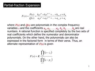
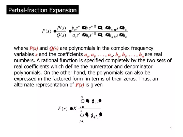
Partial-fraction Expansion where P(s)and Q(s) are polynomials in the complex frequency variables s and the coefficients ao, a1, . . . , an, bo, b1, . . . , bm are real numbers. A rational function is specified completely by the two sets of real coefficients which define the numerator and denominator polynomials. On the other hand, the polynomials can also be expressed in the factored form in terms of their zeros. Thus, an alternate representation ofF(s)is given
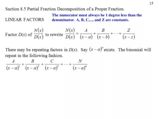
The first step in the partial-fraction expansion is to put the rational function into a proper form. We say that a rational function is proper ifthe degree of the numerator polynomial is less than the degree of the denominator polynomial. If the given rational function F(s)is not proper, i.e.., if the degree of P(s) is greater than or equal to that of Q(s),we divide (long division) P(s) by Q(s)and obtain The quotient, is a polynomial and R(s)is the remainder; therefore, R(s)has a degree less than that of Q(s),and the new rational function R(s)/Q(s)is proper. Since is a polynomial, the corresponding time function is a linear combination of ,(1),(2), etc., and can be determined directly using Tables. We therefore go ahead with the new rational function R(s)/Q(s)which is proper. In the remaining part of this section we assume that all rational functions are proper.
Second Order Polynomial • Roots of Q(s) are called poles and roots of P(s) are called zeros. (polt in the complex frequency domain zeros as ‘o’ and poles as ‘x’) • In general we may write a second order Q(s) as • The roots are • If the damping ratio >1 (roots are real & distinc ‘simple’) • If the damping ratio <1 (roots are complex conjugates • If the damping ratio =1 (roots are real & equal ‘repeated’)
Case 1 Simple poles We start with a simple example as follows: We claim that there are constants K1, K2, and K3such that Heaviside’s Expansion Compare Heaviside’s Expansion with solving for K or substituting convenient values for s.
Case 2 Multiple poles Find the partial-fraction expansion of The function has two multiple poles at s =p1=-1 (third order, n1=3) and at s = p2 = 0 (second order,n2= 2). Thus, the partial fraction expansion is of the form To calculate K11, K12, and K13, we first multiply F(s)by (s +1)3to obtain Using (5-115) we find
Similarly, to calculate K21and K22, we first multiply F(s)by s2to obtain Using (5-115),we find Therefore, the partial-fraction expansion is The corresponding time function is
First, we observe that F(s) is a ratio of polynomials with real coefficients; hence zeros and poles, if complex, must occur in complex conjugate pairs. More precisely, if p1 = 1 + j1is a pole, that is, Q1(p1)=0, then is also a pole; that is, . This is due to the fact that any polynomial Q(s)with real coefficients has the property that for all s. Let us assume that the rational function has a simple pole at s = p1 =-+ j; then it must have another pole at s = p2 = =- - j. The partial-fraction expansion of F(s)must contain the following two terms: Case 3 Complex poles The two cases presented above are valid for poles which are either real or complex. However, if complex poles are present, the coefficients in the partial-fraction expansion are, in general, complex, and further simplification is possible. Using formulafor simple poles, we obtain
Since F(s)is a rational function of s with realcoefficients, it follows that K2 is the complex conjugate of K1. Once K and K* are determined, the corresponding two complex terms can be combined as follows: Suppose K=a+jb. Then K*=a-jb, and Once, we find a and b, given, , using the Inverse Laplace transform, we get
This formula, which gives the corresponding time function for a pair of terms due to the complex conjugate poles, is extremely useful. There are good Matlab examples in your text book utilizing the command residue Practice the examples