Download
1 / 20
200 likes | 206 Views
MANX is a proof-of-principle experiment to demonstrate 6D cooling and exceptional cooling performance for muon colliders. It aims to design a practical helical cooling magnet and explore potential applications for a short-length precooler.

E N D
Design MANX experiment MANX magnet, Matching, and More Katsuya Yonehara NFMCC 2007, UCLA
Aim of the MANX experiment • MANX is a proof-of-principle experiment. • Six dimensional helical cooling theory (ref. PRSTAB 8,041002 (2005) • Demonstrate 6D cooling, Continuous emittance exchange, Exceptional cooling performance… • MANX can be a prototype cooling magnet to R&D of cooling performance for muon colliders • MANX can be applied for a short length precooler. • Synchrotron motion and transverse and longitudinal coupling with the beta function in HCC. • Non-linear effects associated with the higher order EM field components and energy loss process. NFMCC 2007, UCLA
Particle motion in Helical Magnet Combined function magnet (invisible in this picture) Solenoid + Helical dipole + Helical Quadrupole Red: Reference orbit Magnet Center Blue: Beam envelope Dispersive component makes longer path length for higher momentum particle and shorter path length for lower momentum particle. Repulsive force Attractive force Both terms have opposite signs. NFMCC 2007, UCLA
Overview of MANX channel • Use Liquid He absorber • No RF cavity • Length of cooling channel: 3.2 m • Length of matching section: 2.4 m • Helical pitch k: 1.0 • Helical orbit radius: 25 cm • Helical period: 1.6 m • Transverse cooling: ~150 % • Longitudinal cooling: ~120 % • 6D cooling: ~200 % NFMCC 2007, UCLA
Design practical helical cooling magnet See Mike Lamm’s talk Large bore channel (conventional) Small bore channel (helical solenoid) • Siberian snake type magnet • Consists of 4 layers of helix dipole to produce • tapered helical dipole fields. • Maximum field is ~7 T (coil diameter: 1.0 m) • Use helical solenoid coil • Consists of 73 single coils (no tilt). • Maximum field is ~5 T (coil diameter: 0.5 m) • Flexible field configuration NFMCC 2007, UCLA
Helical field maps in TOSCA Small bore magnet (helical solenoid) Large bore magnet (conventional) • Design with l = 2.0 m and k = 0.8 • Design with l = 1.6 m and k = 1.0. NFMCC 2007, UCLA
Natural quadrupole component in small bore magnet system (helical solenoid) • Negative field gradient is produced in helical • solenoid coils. • The required helical quadrupole component is • changed by k (helical pitch). • The strength of the quadrupole component can • be adjusted by the solenoid coil diameter. l = 1.0 m, p = 300 MeV/c NFMCC 2007, UCLA
Matching design • Connect the straight beam section to the helical beam section. • Need to induce • Helical pitch k (=pf/pz) • Helical radius a a NFMCC 2007, UCLA
Adiabatic method Helical section Matching section Helical section Matching section • Use atan to make smooth tapered field. • Clearly see a smooth tracking. • This channel is needed 10~15 meters. NFMCC 2007, UCLA
Can we make a shorter matching section? Repulsive central force Attractive central force • Transverse bj field produces transverse p kick. • Solenoid bz field stabilizes orbit. Equilibrium orbit (ref orbit) a, b, d, and e are the coefficients. NFMCC 2007, UCLA
Shorter matching and HCC field map Upstream M (4 meters) Downstream M (4 meters) HCC (4 meters) Use linear function for first trial Adjust solenoid strength to connect to a proper helical orbit. b0: Amplitude of initial helical dipole magnet a: Ramping rate NFMCC 2007, UCLA
Simulation study Initial beam profile • Beam size (rms): ± 60 mm • Dp/p (rms): ± 40/300 MeV/c • x’ and y’ (rms): ± 0.4 (Acceptance study has not been done yet.) • Obtained cooling factor: ~200% NFMCC 2007, UCLA
Discussion of simulation result • Good cooling performance is preserved in the helical solenoid coil magnet. • Longitudinal betatron oscillation makes complicated emittance evolutions. • Optimize matching magnet • Fine tune Twiss parameters • Optimize MANX magnet • Obtain the best cooling performance. NFMCC 2007, UCLA
Possible beam line in Fermilab site • Candidates • Linac (0.4 GeV proton) See Andreas Jansson’s talk. • Low yield, narrow space • Meson Test area (120 GeV proton) Ask B. Abrams. • Need energy absorber to reduce momentum. • Parasitic design with the ILC detector group • pbar accumulator ring (8 GeV) • Obtain good quality beam, sufficiently high intensity • One of the most preferable place • MiniBooNe (8 GeV) • Need muon capturing element NFMCC 2007, UCLA
Preliminary optics design in MTA See Andreas Jansson’s talk Diagnostic sections HCC 180º dispersion free bend Decay channel Uses BNL D2 quads “Almost” fits in MTA NFMCC 2007, UCLA
Spectrometer design • 6D phase space (or emittance exchange) measurements at HCC entrance/exit are the minimum requirement to verify the cooling theory. • Single particle tracking measurement vs beam measurement • Cost, reliability, precision, beam transport, etc… • Fermilab AD now consider rastering a pencil beam. • The hardest part of the spectrometer design is how to determine the longitudinal phase space. • Time structure measurement? • HCC is a kind of spectrometer itself. Therefore, we can determine the momentum by tracking the particle in HCC. • Other interesting parameter is the feature of isochronous. This can be done by measuring ToF between upstream and downstream spectrometers. • PID? NFMCC 2007, UCLA
Conclusions • Big inflation in magnet design • Found the simple solution for matching • Need fine tuning • Beam line design in progress • Spectrometer design in progress NFMCC 2007, UCLA
Collaborators list Muons, Inc. B. Abrams, M. Alsharo’a, M.A. Cummings, R. Johnson, S. Kahn, M. Kuchnir, T. Roberts JLab K. Beard, A. Bogacz, S. Derbenev IIT D. Kaplan Fermilab Technical Division N. Andreev, V.V. Kashikhin, V.S. Kashikhin, M. Lamm, I. Novitski, V. Yarba, A. Zlobin Fermilab Accelerator Division C. Ankenbrandt, D. Broemmelsiek, M. Hu, A. Jansson, M. Popovic, V. Shiltzsev And many useful comments & suggestions from Muon Collider Task Force people NFMCC 2007, UCLA
Appendix • Show isochronous feature in HCC NFMCC 2007, UCLA
t vs Ptotal MANX Z=0 m t vs Ptotal Z=2 m t vs Ptotal Z=1 m Fractions from initial Dptotal= 0.829 /2m Dptotal= 0.937 /m Dt= 1.002 /2m Dt= 1.001 /m Bin size 0.2 ns t vs Ptotal Z=3 m t vs Ptotal Z=4 m Dptotal= 0.735 /4m Dptotal= 0.762 /3m Dt= 1.005 /4m Momentum compaction factor h = 0.34 gt-2 = 0.72 Dt= 1.003 /3m NFMCC 2007, UCLA