Download
1 / 51
530 likes | 699 Views
Modelling of preferred orientation. László S. Tóth Laboratoire de Physique et Mécanique des Matériaux Université de Metz, France. Outline. Preferred orientation Crystal plasticity Lattice rotation Ideal orientation The case of shear

E N D
Modelling of preferred orientation László S. Tóth Laboratoire de Physique et Mécanique des MatériauxUniversité de Metz, France
Outline • Preferred orientation • Crystal plasticity • Lattice rotation • Ideal orientation • The case of shear • Effect of twinning or dynamic recrystallization on ideal orientations • A Taylor type polycrystal computer program
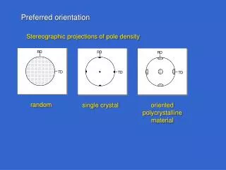
Preferred orientation *Y. Zhou, L.S. Toth, K.W. Neale, "On the stability of the ideal orientations of rolling textures for fcc polycrystals", Acta Metall. et Mat., 40, 3179-3193, 1992.
Crystal plasticity • The comprehension of orientation persistence requires to know the main elements of crystal plasticity. • Distortion of the lattice by elastic strains is neglected in this analysis. • -Dislocation and slip system • Strain equations for slip • Resolution of the strain equations for slip • Strain rate sensitive slip solution • The plastic spin • Lattice rotation • Role of rigid body rotation in lattice spin
n b b Dislocation and slip system Ball-model of a crystal
3 2 1 Strain equations for slip Displacement field: u Eulerian velocity field: Velocity gradient: Introducing the Schmid orientation tensor: Eulerian strain rate tensor:
Resolution of the strain equations for slip Equation system to solve: 5 imposed strain rate components, n unknown slip rates. !Ambiguity problems when the Schmid law is used for n > 5. • Resolution of ambiguities: • regularization of the Schmid law • use of maximum work principle • random selection of 5 slip systems • second order plastic work rate criterion • minimum plastic spin assumption • use self and latent hardening • strain rate sensitive slip • rounding vertices on the yield surface
Strain rate sensitive slip solution Use of constitutive law: m = strain rate sensitivity index Equation system to solve: 5 equations with 5 imposed strain rate components, 5 unknown stress components (use of Newton-Raphson technique to solve) Good initial guess from m = 1 (linear equation system)
Strain rate sensitive slip solution From the obtained deviatoric stress state S, the resolved shear stress is calculated in each slip system: Then the slip rate is obtained from the constitutive law: Verification: the obtained slip distribution has to reproduce the imposed strain rates:
Lattice rotation Three kinds of rotations have to be distinguished: Rigid body rotation rate (material/laboratory): Plastic spin (material/lattice): Lattice spin (lattice/laboratory):
The plastic spin The ‘plastic spin polyhedron’ for {111}<110> slip in the crystal reference system. The rotation vectors are oriented towards the vertices of the polyhedron. Numbers indicate the index of the slip system. At least four slip systems are needed for zero plastic spin. The plastic spin is zero for linear viscous slip (m=1) in f.c.c. crystals for any imposed deformation. Non-zero (but small) for hexagonal crystal symmetry. L.S. Toth, J.J. Jonas, K.W. Neale, "Comparison of the minimum plastic spin and rate sensitive slip theories for loading of symmetrical crystal orientations" (communicated by Rodney Hill), Proc. Roy. Soc. Lond. A427, 201-219, 1990.
plastic spin lattice spin rigid body spin Rigid body rotation zero in rolling, tension, compression. In general, all cases when the velocity gradient is symmetric. In those cases, small lattice spin requires small plastic spin. Small plastic spin is only possible in multiple slip (at least 4 in f.c.c., see plastic polyhedron). Therefore, in rolling, tension and compression the number of necessary operating slip systems for zero or very small lattice spin is four. For simple shear, the rigid body spin is non-zero and very large, consequently, large plastic spin is needed to have zero or small lattice spin. Only one or two slip systems are operating in ideally oriented crystals. Role of rigid body rotation in lattice spin L.S. Toth, P. Gilormini, J.J. Jonas, "Effect of rate sensitivity on the stability of torsion textures", Acta Metall., 36, 3077-3091, 1988.
Orientation updating The lattice spin is obtained from: The orientation of a crystal is described by the transformation matrix T going from the sample to the crystal reference system. Its rate of change is: From this equation: When W is expressed in the crystal axis: When W is expressed in the sample axis: Then, during a small time increment dt:
Ideal orientation Y. Zhou, L.S. Toth, K.W. Neale, "On the stability of the ideal orientations of rolling textures for fcc polycrystals", Acta Metall. et Mat., 40, 3179-3193, 1992.
Ideal orientations in rolling of f.c.c. polycrystals Y. Zhou, L.S. Toth, K.W. Neale, "On the stability of the ideal orientations of rolling textures for fcc polycrystals", Acta Metall. et Mat., 40, 3179-3193, 1992.
Orientation persistence Parameters describing the orientation persistence: 1. Orientation stability parameter, S: 2. Divergence of the rotation field: L.S. Toth, P. Gilormini, J.J. Jonas, "Effect of rate sensitivity on the stability of torsion textures", Acta Metall., 36, 3077-3091, 1988.
Orientation persistence in simple shear L.S. Toth, P. Gilormini, J.J. Jonas, "Effect of rate sensitivity on the stability of torsion textures", Acta Metall., 36, 3077-3091, 1988.
The rotation field in shear L.S. Toth, P. Gilormini, J.J. Jonas, "Effect of rate sensitivity on the stability of torsion textures", Acta Metall., 36, 3077-3091, 1988.
L.S. Toth, K.W. Neale, J.J. Jonas, "Stress response and persistence characteristics of the ideal orientations of shear textures", Acta Metall., 37, 2197-2210, 1989. The divergence in shear
Direction of shear (rigid body rotation) 0 180 0 A1* A2* C 90 Texture evolution in large strain shear g = 2 Key figure for ideal orientations g = 5,5 g = 11 Continuous variations in the texture components in the sense of the rigid body rotation. L.S. Toth, J.J. Jonas, D. Daniel, J.A. Bailey, "Texture development and length changes in copper bars subjected to free end torsion", Textures and Microstructures, 19, 245-262, 1992.
Direction of shear (rigid body rotation) ‘Tilts’ of the components from ideal positions g = 2 L.S. Toth, J.J. Jonas, D. Daniel, J.A. Bailey, "Texture development and length changes in copper bars subjected to free end torsion", Textures and Microstructures, 19, 245-262, 1992.
Direction of shear (rigid body rotation) g = 5.5 L.S. Toth, J.J. Jonas, D. Daniel, J.A. Bailey, "Texture development and length changes in copper bars subjected to free end torsion", Textures and Microstructures, 19, 245-262, 1992.
Direction of shear (rigid body rotation) g = 11 L.S. Toth, J.J. Jonas, D. Daniel, J.A. Bailey, "Texture development and length changes in copper bars subjected to free end torsion", Textures and Microstructures, 19, 245-262, 1992.
Direction of shear (rigid body rotation) Rotation field – C component L.S. Toth, P. Gilormini, J.J. Jonas, "Effect of rate sensitivity on the stability of torsion textures", Acta Metall., 36, 3077-3091, 1988.
Direction of shear (rigid body rotation) Rotation field – C component L.S. Toth, P. Gilormini, J.J. Jonas, "Effect of rate sensitivity on the stability of torsion textures", Acta Metall., 36, 3077-3091, 1988.
Direction of shear (rigid body rotation) Rotation field – C component L.S. Toth, P. Gilormini, J.J. Jonas, "Effect of rate sensitivity on the stability of torsion textures", Acta Metall., 36, 3077-3091, 1988.
Conclusions on main characteristics of large strain shear textures • Continuous variations in the texture components • in the sense of the rigid body rotation, • ‘Tilts’ of the components from ideal positions, • Convergent/divergent nature of the rotation field • around ideal positions, • About 50% of the orientations remain outside of • the ‘tubes’ of the ODF (perpetuel rotation).
Effect of twinning or dynamic recrystallization on ideal orientations Rotated cube Does dynamic recrystallization produce new stable components? simulated Example of shear, measured at 300°C, g=4: J.J. Jonas, L.S. Toth, "Modelling oriented nucleation and selective growth during dynamic recrystallisation", Scripta Met. et Mat., 27, 1575-1580, 1992.
Slip activity-versus DRX Number of active slip systems mapped in the f2=45° Euler space section for simple shear ODF of DRX texture in OFHC copper for simple shear New DRX components (rotated cube) appear at positions with high number of active slip systems (high Taylor factors). These positions, however, have very low orientation stability, so cannot form high ODF intensities.
Modeling of preferred orientation in DRX Observation: high Taylor factor-increases DRX • Mechanisms of DRX: • Oriented nucleation and growth (ONG) • Selective growth into the matrix (SG) Modeling possibilities: 1. Growth of volume fraction of low Taylor factor positions (ONG) 2. Creating nuclei by rotation of parent and growth (SG)
Simplified modeling of DRX Selective growth into the matrix (SG): Nuclei are made by rotating the crystal orientation according to coincident site lattice or plane matching criteria. Example: 40° rotation around plane normal {111} in f.c.c. Then transferring volume fraction from parent to nuclei. Oriented nucleation and growth (ONG): No change in orientation, just volume fraction transfer. A. Hildenbrand, L.S. Toth, A. Molinari, J. Baczynski, J.J. Jonas, "Self consistent polycrystal modelling of dynamic recrystallisation in shear deformation of a Ti-IF steel", Acta Materialia, 47, 447-460, 1999.
Use of volume transfer scheme Eulerian simulation, fix orientation positions in grid points. Variant selection in selective growth: Preferred nuclei pertaining to most active slip system plane.
DRX of IF steel in torsion Experiment Simulation A. Hildenbrand, L.S. Toth, A. Molinari, J. Baczynski, J.J. Jonas, "Self consistent polycrystal modelling of dynamic recrystallisation in shear deformation of a Ti-IF steel", Acta Materialia, 47, 447-460, 1999.
φ2 = 0˚ φ2 = 45˚ φ1 φ1 Φ Pass 1 A1 C A1 C A2 A2 90° A1 Pass 2 C A1 C A2 A2 A A A Pass 3 A1 C A1 C A2 A2 B B B B B B B B B A1 A1 A1 A2 A2 A2 A1 A1 A1 A A A A2 A2 A2 C C C C C C B B B B B B B B B Modeling of preferred orientation in twinning Does twinning produce new stable components? Experimental texture in ECAE of silver: These textures cannot be modeled with slip alone, twinning on {111} planes in <112> directions is necessary. S. Suwas, L.S. Toth, J.J. Fundenberger, A. Eberhardt, W. Skrotzki, "Evolution of crystallographic texture during equal channel angular extrusion of silver", Scripta Materialia, 49, 1203-1208, 2003.
Modeling twinning Twinning is a large shear deformation. In the modeling, its contribution to the total deformation is calculated in the same way as for slip. When twinning is high, slip activity reduced and vice-versa. Twinned part of a grain has new orientation use of volume transfer scheme when all variants are allowed. When only one twin family is admitted to be significativ use of predominant twinning rule (PTR). Parent + twin coexist. Monte Carlo scheme: A parent grain is completely replaced by its twin orientation when twinning activity is high enough, and a random selection is valid. Question: does the twinned part co-rotate with the matrix? In terms of hardening, there is a strong effect of the twin lamellas which reduce the mean free path of dislocation glide (Hall-Petch effect).
φ2 = 0˚ φ2 = 45˚ Taylor Self consistent AE BE BE BE AE A2E A1E CE A2E A1E CE BE BE BE A2E A1E CE A2E A1E CE Simulated twinning activity in silver Twinning activity map: Twinning activity map made for a relative critical stress of 1.10. Isolines: 0.2, 0.4, 0.6, 0.8, 1.0, 1.2, 1.4, where the values mean the sum of cristallographic shears on all twinning systems normalized by the imposed von Mises equivalent strain rate.
φ2 = 0˚ φ2 = 45˚ φ2 = 0˚ φ2 = 45˚ φ1 φ1 φ1 φ1 Φ Φ A Pass 1 Pass 1 A1 B C B A1 B C A2 A2 90° 90° A1 A2 A1 A2 C C A Pass 2 A1 A2 C A1 C A2 A1 Pass 2 C B B A1 B C A2 A2 A1 A2 A1 A2 C C A A A A2 C A2 A1 C A1 A Pass 3 A2 A1 Pass 3 A1 C C A1 A2 C A1 C B B B A2 A2 B B B B B B B B B C C A1 A1 A1 A2 A2 A2 A1 A1 A1 A A A A A A A2 A2 A2 C C C C C C B B B B B B B B B B B B B B B B B B A simulation result for twinning+slip in ECAE of silver: Simulation: Experiment:
Conclusions on simulation of ideal orientation in DRX or twinning DRX or twinning does not produce new persistent ideal orientations. Grain orientations transferred to new orientation position would require convergent slip to remain stable at the new position. Unless the new orientation is not already a stable position, the grain would rotate away. Some new texture components may appear, namely rotated cube, however, they are positions of limited stability and intensity.
A Taylor type polycrystal plasticity code to simulate texture development Input Cubicsys.dat or Hcpsyst.dat Input parameter file Polycr.ctl Input orientation file Main program Polycr.exe Increm.for Output: tauc.out Strength of slip systems/grain Output: stress.out Stress state/grain Output: strain.out Strain state/grain Output: euler.out orientation file
Characteristics of the code A Taylor viscoplastic polycrystal code permetting to simulate texture evolution for any strain mode and any strain. It can be run in full and relaxed constraints conditions with or without hardening. Elasticity is not taken into account. The slip constitutive law is: The program solves the non-linear equation system using Newton-Raphson technique for the deviatoric stress state: Then the resolved shear stresses and the slip rates are calculated from the above first two equations. From the slips, the orientation change is obtained from the equations presented in slide no. 15. Hardening is accounted for using self and latent hardening of the slip systems according to Bronkhorst et al. (1992*): *Bronkhorst, C.A., Kalidindi, S.R. and Anand, L. Phil. Trans. Royal Soc. London, A341, p. 443.
Control parameters - Polycr.ctl Input parameter file Polycr.ctl rand1000.eul ! input file cubicsys.dat ! slip system file, it can only be cubicsys.dat or hcpsyst.dat Pancake rolling of fcc ! title of run 20. ! strain rate sensitivity parameter (1/m) 1 !0: no hardening, 1:Bronkhorst type hard. 10 ! number of increments 0.02 2 1 1 ! strain increment in one step, imode:1:in von Mises, 2: control by index, index1,index2 1 ! 1: constant inposed velocity gradient, 2: variable velocity gradient (from data file velgrad.dat) 1 0 0 ! imposed velocity gradient when it is constant 0 0 0 0 0 -1 0 0 1 ! relaxation matrix 0 0 1 ! put 1 where you want to relax the strain 0 0 0 ! put 0 everywhere for full constraints Taylor deformation mode
Control parameters - Polycr.ctl – cont. Line: strain control in polycr.ctl: -0.02 2 1 1 ! strain increment in one step, imode:1:in von Mises, 2: control by index, index1,index2 The first value is the increment of strain in one step (deps). Attention: it can be negative (compression) or positive (tension). If the next parameter is set to 1, the strain increment is imposed to be a von Mises type strain increment, which is defined from the strain increment tensor as follows: If the second parameter is 2, as in the above example, the strain increment is defined in terms of a specific strain component only. Then, the following two parameters define the first and second index (ij) of the controlled component of the strain tensor.
Control parameters - Polycr.ctl – cont. Velocity gradient in polycr.ctl: The example in the file is: 1 0 0 0 0 0 0 0 -1 It means a plane strain compression (or rolling). The value of 1 means the imposed strain rate, that is 1 s-1. Relaxation matrix in polycr.ctl: The example in the file is: 0 0 1 0 0 1 0 0 0 It means pancake and lath relaxed constraints model in which the shear on plane with normal 3 and in the directions 1 and 2 are relaxed (meaning: will noet be imposed to be 0, they will be calculated from the crystal plasticity solution of the problem.
Control parameters - Input orientation file title what you want second title, if needed random texture generated by RANDTEXT.FOR (23/01/97) :third title 1000 :number of orientations follow 102.74 119.56 33.65 1.0 219.06 36.21 70.51 1.0 166.66 28.59 45.80 1.0 149.74 86.13 38.68 1.0 …… ………… ……… ….. Euler angles are in degrees, in the order: fi1, fi, fi2. Fourth number: relative volume fraction of that orientation.
Control parameters - Input slip system file File: Cubicsys.dat Cubic slip systems hardening parameters: 1. 180. 148. 2.25 : gam0, h0, tausat, a :in case of use of hardening rule by Bronkhorst e al. 1. 1.4 1.4 1.4 : q1: coplanar, q2: colinear, q3: perpendic. ,q4:other :latent hardening parameters (111)<110> .................. 12 : type of family, nr. of systems, do not touch Reference critical resolved shear stress and shear strain (if twinning) : information for next line, the twinning shear value must be 0 for slip systems and equal to the shear associated with twinning, if this is a twinning family. 16. 0. 1 1 1 -1 0 1 1 2 1 1 -1 1 0 1 3 1 1 -1 1 -1 0 4 1 -1 -1 0 1 -1 5 1 -1 -1 1 0 1 6 1 -1 -1 1 1 0 7 1 -1 1 0 1 1 8 1 -1 1 1 0 -1 9 1 -1 1 1 1 0 10 1 1 1 0 1 -1 11 1 1 1 1 0 -1 12 1 1 1 1 -1 0 (110)<111> .................. 12 : A second family, and so on. Reference critical resolved shear stress and shear strain (for twinning) 0. 0.
Organisation of the simulation The main program is polycr.exe. It reads the input parameters and input files and sets up the simulation procedure. The calculation is incremental in strain. One increment is done for all the grains in the sub-program increm.for for one call from polycr.exe. The grain number is limited to 3000 and the total number of slip (or twinning) systems is maximum 48. The maximum number of increments in strain is 2000. When twinning is used, the orientation of a grain is replaced by its twin orientation if sufficient amount of twin occurs (1/3 twin and 2/3 slip) in a grain. Output files: Euler.out: contains the new euler angles of the grains, their volume fractions, and the stability parameter of that orientation. Stress.out: the (Cauchy) stress state for each grain. Strain.out: the strain rate state of each grain at the end of the simulation. Attention: NOT the accumulated finite strain! In full constraints Taylor deformation mode it is the same for each grain (good for checking that the calculation was OK.). It is only interesting if relaxed constraints model is used where the relaxed components will have non-zero values and varying from grain to grain. Tauc.out: the updated new reference strengths of the slip system, in the same order as they are in the input slip system file, for each grain. It is only interesting if hardening was taken into account in the simulation.
Making and plotting of pole figures of the simulated textures The ‘polycr’ software package is complemented by two other softwares for the purpose of visualizing the obtained simulated textures. They are: POLFIG GRAPH4WIN The POLFIG package is to calculate a data file containing the pole figure wanted. This file is ready to be plotted using the GRAPH4WIN package (other software might also be possible to use).
Making and plotting of pole figures of the simulated textures –cont. POLFIG package: The program is polfig.exe. It can use directly the output distribution file of the POLYCR package, named euler.out. Copy first this file into the //POLFIG directory. Edit the polfig.ctl parameter file which controls the pole figure preparation: 1 ! input in form of Euler angles (1) or Miller indices (2) 111 ! which projection: 100, 110, 111, 0001=basal plane hexagonal 3 1 2 ! sequence of projection axes: middle,right,up 2.992 ! radius of pole figure (inch) Line number one must contain: 1, because the pole figure is made from Euler angle positions. (One could also plot from Miller indices). Line number 2 defines the type of projection you want. One type of pole figure (0002) is also possible for hexagonal structure (not others). Third line defines how the axis of the reference system should be positioned. The first number defines the index of the axis what you want in the middle of the pole figure, perpendicular to the sheet. Second number is the index of the axis which is oriented right, horizontal. The third number is the axis which is in the vertical direction (‘up’) on the pole figure. Last row defines the radius of the pole figure in inches. After executing the program polfig.exe, you obtain four data files: Polfig.dat, circle.dat, axisx.dat, axisy.dat. The first contains the positions of the projected poles of the crystal orientations, the second is a file containing the contour circle of the pole figure, the last two ones are just the horizontal and vertical lines of the two visible axes of the reference system.