Download
1 / 1
10 likes | 51 Views
Station Name. Mode 1,2. Mode 3,4. Mode 5,6,7,8. Variance (%). Period (days). Variance (%). Period (days). Variance (%). Period (days). HGOA. 33.1. 55/50. 20.9. 35/33. 21.69. 28-21. HUSF. 31.84. 53/49. 15.74. 36/33. 20.05. 31-20. HIGP. 30.92. 59/54. 18.16. 25/25. 23.77.

E N D
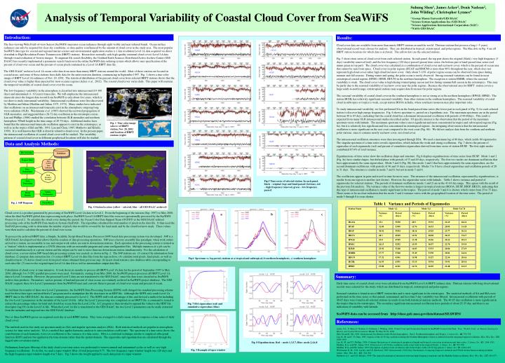
Station Name Mode 1,2 Mode 3,4 Mode 5,6,7,8 Variance (%) Period (days) Variance (%) Period (days) Variance (%) Period (days) HGOA 33.1 55/50 20.9 35/33 21.69 28-21 HUSF 31.84 53/49 15.74 36/33 20.05 31-20 HIGP 30.92 59/54 18.16 25/25 23.77 36-21 HKUS 28.3 49/49 12.91 28/28 20.23 33-17 HWAS 25.0 47/49 13.38 36/26 20.22 20-13 HNSG 24.13 52/52 15.59 36/37 22.70 35-19 HJMS 23.92 51/48 16.03 33/33 20.86 27-19 HMBR 17.77 53/48 15.49 33/30 20.81 24-16 HDUN 17.32 43/41 15.98 31/27 22.54 20-16 HCHL 16.55 63/51 13.15 35/34 19.91 20-14 HPRE 15.88 41/41 14.74 26/29 22.48 22-13 Suhung Shen1, James Acker2, Denis Nadeau2, John Wilding3, Christopher Lynnes4 1 George Mason University/GES DAAC 2 Science System Applications Inc./GES DAAC 3 Science Applications International Corporation (SAIC) 4 NASA GES DAAC Analysis of Temporal Variability of Coastal Cloud Cover from SeaWiFS Introduction: Results: The Sea-viewing Wide Field-of-view Sensor (SeaWiFS) measures ocean radiances through eight visible and near infrared bands. Ocean surface radiances can only be acquired for clear sky conditions, so data quality is influenced by the amount of cloud cover in the study area. The most popular SeaWiFS data type for coastal and regional marine science and environmental application studies is 1-km resolution Level 1A data acquired via direct downlink to High Resolution Picture Transmission (HRPT) stations. Researchers normally seek high-quality (minimal cloud cover) Level 1A data through visual evaluation of browse images. To augment file search flexibility, the Goddard Earth Sciences Distributed Active Archive Center (GES DAAC) has recently implemented a parameter search function in the online SeaWiFS data ordering system which allows user specification of the percent of cloud over ocean and the percent of ocean pixels contained in a Level 1A HRPT data file. The GES DAAC archives Level 1A ocean color data from more than ninety HRPT stations around the world. Most of these stations are located in coastal areas, and some of these stations have daily data for the entire mission duration, commencing in September 1997. Fig. 1 shows a true-color image of HRPT Level 1A radiances of Nov. 20, 2002. The statistical distribution of the percent cloud cover from selected HRPT stations shows that the cloud cover value is higher than expected for most oceanic regions (Acker et al., 2002). The coastal cloud cover varies daily. This paper will examine the temporal variability of coastal cloud cover over the ocean. Cloud cover data are available from more than ninety HRPT stations around the world. Thirteen stations that possess a long (~5 years) observational record were chosen for analysis. They are distributed in tropical, extratropical, and polar regions. The blue dots in Fig. 4 are all HRPT station locations for which data is archived. The yellow dots are the selected stations. Fig. 5 shows time series of cloud cover from each selected station. In each panel, the top part shows the original (black), very high frequency (5 days) variability removed (red), and the low frequency (120 days) passed (green) time series; the bottom part is band-passed time series (red minus green in top part). The cloud cover was calculated as a combination of cloud cover and ice/snow cover, which is the percent of ocean area that cannot be seen from space. Cloud cover in polar regions (HUAF and HMCM) is more than 90% throughout the year, which does not represent high cloud cover rather high cloud/ice/snow cover. Only about 5-10% of polar region oceans can be observed from space during summer and fall seasons. During winter and spring, the polar ocean is rarely observed. Strong seasonal variations can be found in most extratropical coastal regions (HNSG, HJMS, HDUN) in the northern hemisphere. The exception is station HMBR, where the seasonal variability is weak. The cloud cover value is high during winter/spring season and low during summer/fall season in the extratropics. This may be partly due to the seasonal variability of ice/snow cover near the polar regions. Because the observational area for HRPT station covers a large south-to-north range, extratropical stations may acquire data from near the polar regions. The seasonal variability of coastal cloud cover in the southern hemisphere is not as strong as in the northern hemisphere (HWAS, HPRE). The station HCHL has relatively significant seasonal variability than other stations in the southern hemisphere. The seasonal variability of costal cloud in subtropics or tropics is weak, except station HGOA in India, where southeast monsoon may play important roles. To study intraseasonal variability, we first performed SA on the band-passed time series (the lower part in each panel of Fig. 5) for each selected station to discover high energy frequencies. Fig. 6 shows spectrum vs. period on a logarithmic axis. The maximum spectrums are in the period between 40 to 65 days, indicating that the coastal cloud has a dominant intraseasonal oscillation with periods of 40-60days. This result is expected from many OLR intraseasonal studies described earlier. Of specific interest is the observation that the period of the maximum spectrum varies with latitude. The maximum spectrum value is most significant and most concentrated in tropics and sub-tropical regions (Fig. 6a), but it is relatively less significant and less concentrated in extratropical regions. An intriguing observation is that the intraseasonal oscillation is more significant on the east coast compared to the west coast (Fig. 6b). We did not analyze data from the southern and northern polar stations, since it contains mostly ice/snow cover, not cloud cover. The intraseasonal oscillation structures were then investigated through SSA. We used a maximum lag of 80 days, which yields 80 eigenmodes. The singular spectrum of a time series reveals eigenvalues, which indicate the weak and strong oscillations. Fig. 7 shows the percent of eigenvalue of each eigenmode (red) and percent of cumulative eigenvalues derived from time series of station HUSF. The first eight modes contributed 67.6% of total variance. Eigenfunctions of time series show the oscillation shape and structure. Fig.8 displays eigenfunctions of time series from HUSF. Mode 1 and 2 (Fig. 8a) have similar shapes, but shifted phase with periods of 53 and 49 days, respectively. The first two modes are dominant oscillations that have approximately the same eigenvalues. Mode 3 and 4 (Fig. 8b), like mode 1 and 2 that have approximately the same eigenvalues, are the second dominant oscillations, with periods of 36 and 33 days, respectively. Modes 5 to 8 have closed eigenvalues and oscillation periods of 20 to 31 days. The structure is similar in mode 7 and 8, but not in mode 5 and 6. The oscillations appear in pairs and travel in time for most cases. The structure of the intraseasonal oscillation, represented by eigenfunctions, is similar from one region to another (not shown). However, the eigenvalue varies with latitude. Table 1 shows variance and period of eigenmodes for selected stations. The periods of dominant oscillations (mode 1 and 2) are in the 41-63 day range. This agrees with the result of the previous SA analysis. The variance value of the first two modes is largest in tropical stations (HGOA, HUSF, HIGP, HKUS), indicating that this type of intraseasonal oscillation is mostly significant in the tropics. The period of mode 3 and 4 is shorter, which varies from 25 to 37 days. There seems to be no clear indication that the mode 3 and 4 variance varies with the geographical location of the time series. The period of mode 5 through 8 is even shorter. The low-frequency variability in the atmosphere is classified into intraseasonal (10-100 days) and interannual (1- 10 years) timescales. We will emphasize the intraseasonal timescale since the longest data record from SeaWiFS is only about five years, which is too short to study interannual variability. Intraseasonal oscillations were first discovered by Madden and Julian (Madden and Julian, 1971, 1972). Many studies have indicated that oscillations on an intraseasonal timescale exist in the atmospheric outgoing long wave radiation (OLR). Weickmann et al. (1985) showed the eastward propagation of OLR anomalies, and suggested that a 28-72 day oscillation in the extratropics exists. Lau and Phillips (1986) studied the correlation between OLR anomalies and northern hemisphere 500mb height in the time range of 20-70 days. Additional studies have found that the intraseasonal timescale oscillation appears to exist in the extratropics, as well as in the tropics (Ghil and Mo, 1991; Lau and Chan, 1985; Matthews and Kiladis, 1999). It is well known that OLR is directly related to cloud cover. In the present paper, the intraseasonal oscillation of coastal cloud cover will be studied. The variability patterns of coastal cloud cover in different geophysical locations will also be studied. Fig. 1 True color image (above) of HRPT station, Nov. 20, 2002 and location of HRPT stations (right) Data and Analysis Methods: Database File Selection Prepare Data Data Archive Tape Library Data Extraction Disk Resource Manager Data Processing Fig.5 Time series of selected station. In each panel, black – original (top) and band passed (bottom), red – high frequency removed, green – low frequency passed. Update Parameters Read Results Fig. 2 S4P Diagram Clean Data Table 1 Variance and Periods of Eigenmodes Fig. 4 Station location (yellow – selected, blue – all GES DAAC archived) Cloud cover is a product generated by processing of SeaWiFS Level 1A data to Level 2. From the beginning of the mission (Sep. 1997) to May 2000, when the third SeaWiFS global data reprocessing took place, SeaWiFS Level 1A HRPT data files were not operationally processed by the SeaWiFS Project to Level 2. To calculate the cloud cover during this period, the Ocean Color Data Support Team (OCDST) at the GES DAAC utilized processing code of the SeaWiFS Data Analysis System (SeaDAS). The algorithm calculated the total number of pixels in the data file. It then used the SeaDAS processing code to determine the number of pixels that would be covered by the land mask and by the cloud/ice/snow mask. These values were then used to calculate the percent of cloud over ocean. To process the archived HRPT data, a Simple, Scalable, Script-Based Science Processor (S4P) based data processing system was developed. S4P is a GES DAAC developed tool that allows flexible creation of data processing operations. S4P uses a factory assembly line paradigm: when work orders arrived at a station, an executable is run, and output work orders are sent to downstream stations. Each operation in the processing system is termed as a “station” which is implemented as a UNIX directory with an executable program and some configuration files. Multiple instances of a job can be executed simultaneously at a given station and the output can be sent to more than one downstream station simultaneously. For the calculation of cloud cover, a seven-station S4P-based data processing system was created, as shown in Fig. 2. The S4P stations are (1) extract file information from database; (2) prepare data extraction list; (3) extract HRPT Level 1A data files from the tape archive; (4) calculate total pixels, land pixels, as well as cloud/ice/snow; (5) derive cloud cover from pixel values obtained from previous step; (6) insert cloud statistics into database table corresponding to each data file; (7) remove the original input Level 1A data file as well as intermediate output data files. Calculation of cloud cover is time-intensive. It took about six months to process all HRPT Level 1A data for the period of September 1997 to May 2000, although 3 to 5 CPU parallel processors were used. Fortunately, starting from May 2000, the SeaWiFS project processes all HRPT Level 1A data to Level 2 routinely. However, the processed Level 2 data are not transferred to the GES DAAC, since this data is not classified as SeaWiFS archive data products. Parameters, such as percent of land and percent of clear ocean, are routinely archived in SeaWiFS project database. The GES DAAC requests these two Level 2 parameters from SeaWiFS Project and converts them to percent of cloud over ocean and percent of ocean. To facilitate the transfer of these two Level 2 parameters, the SeaWiFS Data Processing System (SDPS) staff changed the standard processing scheme used for these data types and modified a C program used to manipulate the file descriptor in an HDF file. Although the SDPS only sends Level 1A HRPT data to the GES DAAC, the data are routinely processed to Level 2. The SDPS staff took advantage of this and devised a method for including the two Level 2 parameters in the metadata of the Level 1A file. After the Level 2 processing was completed on an HRPT file, a command is issued to extract the percentage values for land and cloud-free ocean from the Level 2 file. A C program is then invoked to append the values to the HDF file descriptor (tag101) in the Level 1A file. When the Level 1A file is transferred to the GES DAAC, the two Level 2 parameters can be easily extracted from the metadata and ingested into the GES DAAC database. Two or three SeaWiFS passes are acquired each day at each HPRT station. They were averaged to a daily mean, which composes a time series of daily cloud cover. The methods used in this study are spectrum analysis (SA) and singular spectrum analysis (SSA). Both statistical methods are popular in atmospheric science for time series analysis. SA is a method that applies harmonic analysis to autocorrelation coefficients. The spectrum of a time series shows the contributions of each harmonic wave (or oscillation) to the variance of a time series. SSA is a statistical technique similar to empirical orthogonal function (EOF) analysis but applied on the time domain rather than the spatial domain. The eigenvalue and eigenfunction are calculated through the lagged auto-covariance matrix. Preliminary band pass filtering of the daily cloud cover time series was performed to remove annual and semiannual cycles as well as very high frequency oscillations. To do this, we used a taper window filter of total proportion 0.75. The low frequency taper window length was 120 days and the high frequency taper window length was 5 days. Fig.3 shows the weight applied to each data point of a taper window. a b c Fig.6 Spectrum vs. log period, stations at a) tropical and subtropical, b) northern hemispheric, c) southern hemisphere Summary: Daily time series of coastal cloud cover were calculated from SeaWiFS Level 1A HRPT radiance data. Thirteen stations with long observational records were selected for the study, which are distributed in tropical, extratropical and polar regions. Seasonal variation is found in most HRPT station data and is most significant in the extratropics. The statistical methods of SA and SSA were performed on the time series so that annual, semiannual, and less than 5 day variability was filtered. Intraseasonal oscillations with periods of 40-65 days were found in all selected stations in results from both statistical analysis methods. The 40-65 day oscillation is more significant in the tropics than in the extratropics. The secondary significant intraseasonal oscillations have periods of about 25-35 day, and there is no indication of variability with latitude. SeaWiFS data can be accessed from http://daac.gsfc.nasa.gov/data/dataset/SEAWIFS/ Fig. 7 SSA eigenvalues (red) and cumulative eigenvalues (blue) References: Acker, J.G., S. Shen, D. Nadeau, G. Feldman, J. Wilding, 2002: Cloud Cover and Ocean Area Search for SeaWiFS Ocean Color Data. Proc. 7th Intl. Conf. on Remote Sensing for Marine and Coastal Environments, Miami, Fl, May 20-22, 2002. Ghil, M and K. Mo, 1991: Intraseasonal Oscillations in the Global Atmospheric. Part I: Northern hemisphere and Tropics. J. Atmos Sci., 48, 752-778 Lau, K.-M. and C. P. Chan, 1985: Aspects of the 40-50 day oscillation during the Northen Hemisphere winter as inferred from the outgoing longwave radiation. Mon. Wea. Rev., 113, 1889-1909. Lau, K.-M. and T.J. Phillips, 1986: Coherent fluctuations of extratropical geophysical height and tropical convection in intraseasonal time scales. J. Atmos. Sci., 43., 1164-1181. Madden, R.A. and P.R., Julian, 1971: Detection of a 40-50 day oscillation in the zonal wind in the tropical Pacific. J. Atmos. Sci., 28, 702-708. Madden, R.A. and P.R. Julian, 1972: Description of global-scale circulation cells in the tropics with a 40-50 day period. J. Atmos. Sci., 29, 1109-1123. Weickmann K. M., G.R. Lussky, and J.E. Kutzbach, 1985: Intraseasonal (30-60 day) fluctuations of outgoing longwave radiation and 250mb stream-function during northern winter. Mon. Wea. Rev., 113, 941-961 Matthews A.J., and G.N. Kiladis, 1999: The tropical-extratropical interaction between high-frequency transients and the Madden-Julian oscillation, Mon. Wea. Rev., 127, 661-677. Fig. 8 Eigenfunctions. Red – mode 1,3,5,7; Blue- mode 2,4,6,8 Fig. 3 Example of taper window