Download
1 / 24
240 likes | 332 Views
Energy & Helicity Flux into the Corona. I’ll discuss secular trends , ‘the relatively consistent movement of a variable over a long period’ – ‘DC’ as opposed to ‘AC’ (wave) flux I’ll assume ideal MHD applies, E = -( v x B )/c First, express fluxes in equations…

E N D
Energy & Helicity Flux into the Corona • I’ll discuss secular trends, ‘the relatively consistent movement of a variable over a long period’ – ‘DC’ as opposed to ‘AC’ (wave) flux • I’ll assume ideal MHD applies, E = -(v x B)/c • First, express fluxes in equations… • …then in terms of boundary motions that • we all know and love!
Energy Flux • Poynting Flux, with E = -(v x B)/c: • Rewrite using BAC – CAB rule, take z-comp: (*) (*)
Emergence of Energy • Archetype is vertical, perpendicular flow – e.g., vz advecting a flux tube’s apex (*) • NB: does not include vertical, parallel flow – e.g., continued emergence of a “U-bolt” (*)
Emergence of Free Energy (EF) • EF from emerging non-potential fields (*) related to helicity emergence • EF from shearing or twisting (*) propagation of twist (*) (cf., Nightingale’s rotating sunspots) • possibly from emerging potential fields into potential background fields! Depends on global topology! (*)
Relative Helicity, Defined • Refers to two B-fields and their vector potentials: • B is the actual magnetic field, which may or may not vanish (Bn 0) on the boundary V of V. • BP is the current-free magnetic field that matches the actual field Bn on the boundary. • A is a vector pot’l for B, B = ( x A), and AP is vector pot’l for BP (“potential field’s potential”). • In the general case (barring symmetry), B BP H 0. • This helicity is gauge invariant (Berger & Field, 1984).
Vector Potential, AP • By construction, n· ( x A) = Bz , (·AP)= 0, and (AP· n) = 0. • Regions of Bz 0 on the photosphere are sources of AP, which is a 2-D vector field. • AP is circumferential (*), and completely specified by Bz – knowing Bh unnecessary!
Helicity Flux – Poynting-like Eqn. • From Faraday’s Law for B/t , and assuming A/t = -cE = (v x B), Berger & Field computed dH/dt across a surface (z = normal direction) • Rz is a helicity flux density (Mx2/cm2/s).
Emergence of Helicity • Emergence of helicity-carrying (“helical”— basically, twisted!) fields. (*) • e.g., current-carrying fields observed by Leka et al. (1996) • Emergence of non-helical (potential) fields, resulting in non-potential topology! Depends on global topology! (*)
Helicity Flux by Shearing/Twisting • Motion of magnetic flux along contours of AP leads to a flux of helicity. (*) • Contours are circular, so relative circular motion, a.k.a., braiding, leads to helicity injection. • Propagation of twist along flux tube (*) should lead to observable foot point braiding.
Q. How can we determine the photospheric velocity? • (Not just any photospheric velocity – we want the velocity that affects the photospheric magnetic field.) • Doppler info can give LOS velocity, e.g., Chae (2004) • Local Correlation Tracking (LCT), e.g., Chae (2001) • Newer methods: Kusano et al. (2002), ILCT, MEF, Minimum Structure, ??? • More at Velocity Shootout in WG1 splinter session on Fri!
Démoulin & Berger’s (2003) Hypothesis • LCT applied to Bz or BLOS from photospheric magnetograms gives the pattern velocity. • Pattern velocity uLCT is related to plasma velocity v by: dE/dt and dH/dt can be written in terms of (uLCT Bz)!
dE/dt and dH/dt in terms of uLCT Bz • From LCT on vector magnetograms, can compute fluxes of magnetic energy and helicity. • With LOS magnetograms, and an assumed Bh (e.g., FFF that matches coronal observations), can estimate energy & helicity fluxes.
Helicity & Energy Fluxes • Barring symmetry, if B BP, then H 0. |dH/dt| > 0 B BP • Since BP is unique, and minimum energy given Bz(x,y), B BPalso means free energy is present, EF 0. • Knowledge of Bz specifies AP. • Knowledge of v allows computation of dE/dt & dH/dt.
Emerging Omega Loop (BACK)
“Trombone Slide” Emergence (BACK)
Vector Potential Pictorial (BACK)
Vector Potential Pictorial (BACK)
Vector Potential Pictorial (BACK)