Download

1 / 30
310 likes | 598 Views
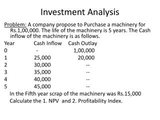
Investment Analysis. Lecture: 10 Course Code: MBF702. Outline. RECAP Risk Analysis in investment analysis Techniques for risk analysis. Comparing Methods. Risk in Investment Appraisal. Risk: refers to a situation where the future is unclear and there is more than one possible outcomes.

E N D
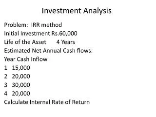
Investment Analysis Lecture: 10 Course Code: MBF702
Outline • RECAP • Risk Analysis in investment analysis • Techniques for risk analysis
Risk in Investment Appraisal Risk: refers to a situation where the future is unclear and there is more than one possible outcomes.
Techniques for dealing with Risk • The techniques for dealing with risk include: a) the expected NPV rule; b) the risk-adjusted discount rate approach; c) sensitivity analysis d) Simulation e) Scenario Analysis
Expected Net Present Value The expected NPV rule (ENPV): • EV of a project is the mean value which will be obtained if the project was repeated many times over • EV is not the most likely value of the project. • It is only the weighted average of all the possible outcomes • EV is calculated by multiplying the each possible outcome by its probability of occurrence and then add them up
Example • Shorten Ltd needs to purchase a machine to manufacture a new product. The choice lies between two machines (A and B). Each machine has an estimated life of three years with no scrap value. • Machine A will cost £30,000 and machine B will cost £40,000, payable immediately in each case. The total variable cost of manufacture of each unit are £2 if made on machine A, but only £1.00 if made on machine B. This is because machine B is more sophisticated and requires less labour to operate it. • The product will sell for £8 each. • The demand for the product is uncertain but is estimated at 2,000 units for each year, 3,000 units for each year or 5,000 units for each year. (Note that whatever sales level actually occurs, that level will apply to each year.) • The sales manager has placed probabilities on the level of demand as follows:
Shorten Ltd:Example Annual demand Probability of occurrence 2000 0.2 3000 0.6 5000 0.2 Presume that both taxation and fixed costs will be unaffected by any decision made. Shorten Ltd’s cost of capital is 6% p.a. • Calculate the NPV for each of the three activity levels for each machine A and B and state your conclusion. • Calculate the expected NPV for each machine and state your conclusion.
Shorten Ltd:Example Machine A 2000 3000 5000 DemandDemandDemand £ £ £ • Year 0 (30,000) (30,000) (30,000) • 1 (£8-£2)/unit 12,000 18,000 30,000 • 2 12,000 18,000 30,000 3 12,000 18,000 30,000 • Discounted : Factor • £ £ £ • Year0 (1.00) (30,000) (30,000) (30,000) • 1 (0.94) 11,280 16,920 28,200 2 (0.89) 10,680 16,020 26,700 • 3 (0.84) 10,080 15,120 25,200 • £2,040 £18,060 £50,100 • Expected value • = (0.2 x 2,040) + (0.6 x 18,060) + (0.2 x 50,100) • = £21,264
Solution Different cash flows of Machine B 2000 3000 5000 DemandDemandDemand £ £ £ Year 0 40,000 40,000 40,000 1(£8-£1)/unit 14,000 21,000 35,000 2 14,000 21,000 35,000 3 14,000 21,000 35,000
Solution Demand: 2000 3000 5000 Discounted : Factor £ £ £ Year0 (1.00) (40,000) (40,000) (40,000) 1 (0.94) 13,160 19,740 32,900 2 (0.89) 12,460 18,690 31,150 3 (0.84)11,760 17,640 29,400 (£2,620) £16,070 £53,450 Expected value = (0.2 x 2,620) + (0.6 x 16,070) + (0.2 x 53,450) = £19,808
The Risk Adjusted Discount Rate This approach to investment decision making process is an attempt to deal with risk in a manner that takes account of the attitudes of the decision maker.
The Risk Adjusted Discount Rate Example 4.2 • Before any investments are considered, the decision maker should begin by determining an appropriate discount rate for risk-free investments. • Suppose that the rate on such bonds issued by the government is currently 7%. This figure should be used as the base from which discount rates are calculated for risky investments.
The Risk Adjusted Discount Rate Class of Risk Example of Risk Premium Discount rate type of project • Very low Buying a bond 1% 8% • Low Improvement in Existing factory 3% 10% • Medium Increased in existing Output 5% 12% • High Launch a new product 8% 15% • Very high Research on areas Related to current activity 11% 18% • The use of risk-adjusted discount rate approach to investment appraisal is indeed, a common sense approach. However, it is subjective, particularly, the choice of the risk premiums and the assignment of projects to particular risk classes is based on personal judgement.
Sensitivity Analysis • Sensitivity analysis: • is a procedure that calculates the changes in the net present value given a change in one of the cash flow elements such as product price. • With sensitivity analysis each of the figures used in the NPV is examined in turn, to determine how variations from the estimated figures impact on the NPV
Sensitivity Analysis • Sensitivity analysis helps managers to gain better understanding of the nature and degree of risk associated with a project; • because it reveals the margin of safety associated with each key variable relating to a particular project. • It is a form of break even analysis. The point at which NPV is equal to zero is the break-even point.
Sensitivity Analysis Identifying the key or critical variable i.e. those with short margin of safety.
Sensitivity Analysis – Formulas • Selling Price: NPV / Present Value of Sales • Sales Volume: NPV / Present Value of CM • Variable cost: NPV / Present Value of Variable Cost • Fixed Cost: NPV / Present Value of Fixed Cost • Cost / Initial Investment: NPV / Present Value of Investment • Discount Rate: IRR • Project Life: ( Total Life - Discounted Payback Period)/ total life
Sensitivity analysis - Question Swift Ltd, which has a cost of capital of 12 per cent, is considering the investment of £7m in an improved moulding machine project with a life of four years. The garden ornaments produced will retail at £9.20 each and cost £6 each to make. It is expected that 800,000 ornaments will be sold each year. What are the key variables for the project?
Sensitivity analysis - Solution NPV of the project can be expressed in terms of the project variables as follows: NPV = ( (S -VC) X CPVF.) – I0 Where: S = Selling price per unit VC = Variable cost per unit N = No of units sold per year I0 = initial investment CPVF. = Cumulative present value factor for four years at 12%
Sensitivity analysis - Solution Inserting the information given in the question and finding the cumulative PV factor from annuity table, we have: (9.20 - 6.00) X800,000X 3.037)-7,000,000 = 0
Sensitivity analysis (a) Initial investment • Initial investment. Find the value of I0 that makes the NPV zero I0 = (9.20 -6.00) x 800,000 x 3.037) = £7,774,720 This is an increase of £774,720 or 11.1 per cent on the planned initial investment
Sensitivity analysis (b) sales price (c) variable cost b) Sales price S = 6.00 + (7,000,000 / (800,000 x 3.037) ) = £8.88 This is a decrease of 32 pence or 3.5 per cent of planned sales price. • Variable cost As a decrease of 32 pence in sales price makes the NPV zero, an increase of 32 pence or 5.3 per cent in variable cost will have the same effect.
Sensitivity analysis (d) Sales volume d). Sales volume N = 700,000 / (9.20 - 6.00) x 3.037) = 720,283 • This is a decrease of 79,717 units or 10 per cent on the planned sales volume.
Sensitivity analysis (e) Discount rate CPVF = 7,000,000 / (9.20 – 6.00) X 800,000) = 2.734 • Using the annuity tables 2.743 corresponds to the discount rate of almost exactly 17 per cent. An increase of 5 per cent in absolute terms or 42 per cent on the current project discount rate.
Sensitivity analysis- Solution summary Sensitivity analysis of the proposed investment by Swift Ltd Variable Original est. B/E point Difference Dif. as % Sensitivity • Sales Volume 800,000 720,283 (79,717) 10% Low • Sales price £9.20 £8.88 (£0.32) 3.5% High • Variable cost £6.00 £6.32 £0.32. 5.3% High • Discount rate 12% 17% 5% 42% Very Low • Initial Inv £7,000,000 £7,774,720 £774,720 11.1% Low
Advantages and Disadvantages Advantages • Useful in directing the attention of managers to the most sensitive variables of the project Disadvantages • Does not formally quantify risk • Does not clearly provide any clear-cut decision rule
Sensitivity analysis- summary • Sensitivity analysis is one method of analyzing the risks surrounding capital expenditure project & enables an assessment to be made of how responsive the project NPV is to changes in the variables used to calculate that NPV. • A sensitivity analysis calculates the consequences of incorrectly estimating a variable in your NPV analysis. • It forces you: • To identify the variables underlying your analysis. • To focus on how changes to these variables could impact the expected NPV. • To consider what additional information should be collected to resolve uncertainties about the variables.
Scenario Analysis • A scenario analysis involves changing several variables at once in your NPV forecast.
Simulation • Simulation Analysis • A simulation analysis uses a computer to generate hundreds, or even thousands, of possible scenarios. • A probability distribution is assigned to each combination of variables to create an entire range of potential outcomes.