Download
1 / 111
2.04k likes | 3.73k Views
The Islamic University of Gaza Faculty of Engineering Civil Engineering Department Hydraulics - ECIV 3322. Water Flow in Pipes. Chapter 3. 3.1 Description of A Pipe Flow. Water pipes in our homes and the distribution system

E N D
The Islamic University of GazaFaculty of EngineeringCivil Engineering DepartmentHydraulics - ECIV 3322 Water Flow in Pipes Chapter 3
3.1 Description of A Pipe Flow • Water pipes in our homes and the distribution system • Pipes carry hydraulic fluid to various components of vehicles and machines • Natural systems of “pipes” that carry blood throughout our body and air into and out of our lungs.
Pipe Flow: refers to a full water flow in a closed conduits or circular cross section under a certain pressure gradient. • The pipe flow at any cross section can be described by: • cross section (A), • elevation (h), measured with respect to a horizontal reference datum. • pressure (P), varies from one point to another, for a given cross section variation is neglected • The flow velocity (v), v = Q/A.
Difference between open-channel flow and the pipe flow • Pipe flow • The pipe is completely filled with the fluid being transported. • The main driving force is likely to be a pressure gradient along the pipe. • Open-channel flow • Water flows without completely filling the pipe. • Gravity alone is the driving force, the water flows down a hill.
Types of Flow • Steady and Unsteady flow The flow parameters such as velocity (v), pressure (P) and density (r) of a fluid flow are independent of time in a steady flow. In unsteady flow they are independent. For a steady flow For an unsteady flow If the variations in any fluid’s parameters are small, the average is constant, then the fluid is considered to be steady
Uniform and non-uniform flow A flow is uniform if the flow characteristics at any given instant remain the same at different points in the direction of flow, otherwise it is termed as non-uniform flow. For a uniform flow For a non-uniform flow
Examples: • The flow through a long uniform pipediameter at a constant rate is steadyuniform flow. • The flow through a long uniform pipediameter at a varying rate is unsteadyuniform flow. • The flow through a diverging pipediameter at a constant rate is a steadynon-uniform flow. • The flow through a diverging pipediameter at a varying rate is an unsteadynon-uniform flow.
Laminar flow: • Laminar and turbulent flow The fluid particles move along smooth well defined path or streamlines that are parallel, thus particles move in laminas or layers, smoothly gliding over each other. Turbulent flow: The fluid particles do not move in orderly manner and they occupy different relative positions in successive cross-sections. There is a small fluctuation in magnitude and direction of the velocity of the fluid particles transitional flow The flow occurs between laminar and turbulent flow
3.2 Reynolds Experiment Reynolds performed a very carefully prepared pipe flow experiment.
Reynolds Experiment • Reynold found that transition from laminar to turbulent flow in a pipe depends not only on the velocity, but only on the pipe diameter and the viscosity of the fluid. • This relationship between these variables is commonly known as Reynolds number (NR) It can be shown that the Reynolds number is a measure of the ratio of the inertial forces to the viscous forces in the flow
Reynolds number where V: mean velocity in the pipe [L/T] D: pipe diameter [L] : density of flowing fluid [M/L3] : dynamic viscosity [M/LT] : kinematic viscosity [L2/T]
It has been found by many experiments that for flows in circular pipes, the critical Reynolds number is about 2000 Flow laminar when NR < Critical NR Flow turbulent when NR > Critical NR The transition from laminar to turbulent flow does not always happened at NR = 2000 but varies due to experiments conditions….….this known as transitional range
Laminar Vs. Turbulent flows • Laminar flows characterized by: • low velocities • small length scales • high kinematic viscosities • NR < Critical NR • Viscous forces are dominant. • Turbulent flows characterized by • high velocities • large length scales • low kinematic viscosities • NR > Critical NR • Inertial forces are dominant
Example 3.1 40 mm diameter circular pipe carries water at 20oC. Calculate the largest flow rate (Q) which laminar flow can be expected.
3.3 Forces in Pipe Flow • Cross section and elevation of the pipe are varied along the axial direction of the flow.
For Incompressible and Steady flows: Conservation law of mass Mass enters the control volume Mass leaves the control volume Continuity equation for Incompressible Steady flow
Apply Newton’s Second Law: Fx is the axial direction force exerted on the control volume by the wall of the pipe. Conservation of moment equation
Example 3.2 dA= 40 mm, dB= 20 mm, PA=500,000 N/m2, Q=0.01m3/sec. Determine the reaction force at the hinge.
3.4 Energy Head in Pipe Flow Water flow in pipes may contain energy in three basic forms: 1- Kinetic energy, 2- potential energy, 3- pressure energy.
Consider the control volume: • In time interval dt: - Water particles at sec.1-1 move to sec. 1`-1` with velocity V1. - Water particles at sec.2-2 move to sec. 2`-2` with velocity V2. • To satisfy continuity equation: • The work done by the pressure force ……. on section 1-1 ……. on section 2-2 -ve sign because P2 is in the opposite direction to distance traveled ds2
The work done by the gravity force : • The kinetic energy: The total work done by all forces is equal to the change in kinetic energy: Dividing both sides by rgQdt Bernoulli Equation Energy per unit weight of water OR: Energy Head
Energy head Kinetic head Pressure head Elevation head = + + • Notice that: • In reality, certain amount of energy loss (hL) occurs when the water mass flow from one section to another. • The energy relationship between two sections can be written as:
ExampleIn the figure shown:Where the discharge through the system is 0.05 m3/s, the total losses through the pipe is 10 v2/2g where v is the velocity of water in 0.15 m diameter pipe, the water in the final outlet exposed to atmosphere.
Calculate the required height (h =?) below the tank
Energy Losses (Head losses) Major Losses Minor losses Calculation of Head (Energy) Losses: In General: When a fluid is flowing through a pipe, the fluid experiences some resistance due to which some of energy (head) of fluid is lost. Loss due to the change of the velocity of the flowing fluid in the magnitude or in direction as it moves through fitting like Valves, Tees, Bends and Reducers. loss of head due to pipe friction and to viscous dissipation in flowing water
3.5 Losses of Head due to Friction • Energy loss through friction in the length of pipeline is commonly termed the major loss hf • This is the loss of head due to pipe friction and to the viscous dissipation in flowing water. • Several studies have been found the resistance to flow in a pipe is: - Independent of pressure under which the water flows - Linearly proportional to the pipe length, L - Inversely proportional to some water power of the pipe diameter D - Proportional to some power of the mean velocity, V - Related to the roughness of the pipe, if the flow is turbulent
Major losses formulas • Several formulas have been developed in the past. Some of these formulas have faithfully been used in various hydraulic engineering practices. • Darcy-Weisbach formula • The Hazen -Williams Formula • The Manning Formula • The Chezy Formula • The Strickler Formula
The resistance to flow in a pipe is a function of: • The pipe length, L • The pipe diameter, D • The mean velocity, V • The properties of the fluid () • The roughness of the pipe, (the flow is turbulent).
Darcy-Weisbach Equation Where: fis the friction factor L is pipe length D is pipe diameter Q is the flow rate hL is the loss due to friction It is conveniently expressed in terms of velocity (kinetic) head in the pipe The friction factor is function of different terms: Renold number Relative roughness
Friction Factor: (f) • For Laminar flow: (NR < 2000) [depends only on Reynolds’ number and not on the surface roughness] • For turbulent flow in smooth pipes (e/D = 0) with 4000 < NR < 105 is
For turbulent flow ( NR > 4000 ) with e/D > 0.0, the friction factor can be founded from: • Th.von Karman formulas: • Colebrook-White Equation for f There is some difficulty in solving this equation So, Miller improve an initial value for f , (fo) The value of fo can be use directly as f if:
Friction Factor f laminar flow NR < 2000 e e e pipe wall pipe wall pipe wall The thickness of the laminar sublayer d decrease with an increase in NR f independent of relative roughness e/D Smooth f varies with NR and e/D transitionally rough Colebrook formula turbulent flow f independent of NR rough NR > 4000
Moody diagram • A convenient chart was prepared by Lewis F. Moody and commonly called the Moody diagram of friction factors for pipe flow, There are 4 zones of pipe flow in the chart: • A laminar flow zone where f is simple linear function of NR • A critical zone (shaded) where values are uncertain because the flow might be neither laminar nor truly turbulent • A transition zone where fis a function of both NR and relative roughness • A zone of fully developed turbulence where the value of f depends solely on the relative roughness and independent of the Reynolds Number
Laminar Marks Reynolds Number independence
Typical values of the absolute roughness (e) are given in table 3.1
Notes: • Colebrook formula is valid for the entire nonlaminar range (4000 < Re < 108) of the Moody chart In fact , the Moody chart is a graphical representation of this equation
Problems (head loss) Three types of problems for uniform flow in a single pipe: • Type 1: • Given the kind and size of pipe and the flow rate head loss ? • Type 2: • Given the kind and size of pipe and the head loss flow rate ? • Type 3: • Given the kind of pipe, the head loss and flow rate size of pipe ?
Example 1 The water flow in Asphalted cast Iron pipe (e = 0.12mm) has a diameter 20cm at 20oC. Is 0.05 m3/s. determine the losses due to friction per 1 km • Type 1: • Given the kind and size of pipe and the flow rate head loss ? Moody f = 0.018
Example 2 The water flow in commercial steel pipe (e = 0.045mm) has a diameter 0.5m at 20oC. Q=0.4 m3/s. determine the losses due to friction per 1 km • Type 1: • Given the kind and size of pipe and the flow rate head loss ?
Use other methods to solve f 1- Cole brook
Example 3 Cast iron pipe (e = 0.26), length = 2 km, diameter = 0.3m. Determine the max. flow rate Q , If the allowable maximum head loss = 4.6m. T=10oC • Type 2: • Given the kind and size of pipe and the head loss flow rate ?
Trial 1 Trial 2 V= 0.82 m/s , Q = V*A = 0.058 m3/s
Compute the discharge capacity of a 3-m diameter, wood stave pipe in its best condition carrying water at 10oC. It is allowed to have a head loss of 2m/km of pipe length. Example 3.5 • Type 2: • Given the kind and size of pipe and the head loss flow rate ? Solution 1: Table 3.1 : wood stave pipe: e = 0.18 – 0.9 mm, take e = 0.3 mm At T= 10oC, n = 1.31x10⁻⁶ m2/sec