Download
1 / 29
290 likes | 515 Views
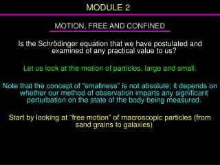
MODULE 2. MOTION, FREE AND CONFINED Is the Schrödinger equation that we have postulated and examined of any practical value to us? Let us look at the motion of particles, large and small.

E N D
MODULE 2 MOTION, FREE AND CONFINED Is the Schrödinger equation that we have postulated and examined of any practical value to us? Let us look at the motion of particles, large and small. Note that the concept of “smallness” is not absolute; it depends on whether our method of observation imparts any significant perturbation on the state of the body being measured. Start by looking at “free motion” of macroscopic particles (from sand grains to galaxies)
MODULE 2 Consider a ball that can move in the x-dimension, without potential energy barriers, i.e., V(x) = 0. Like this: and not like this Where V1, V2 > 0 Our ball has a mass m and velocity v in either direction (+x or -x).
MODULE 2 The object is a macro-entity and so we can determine its instantaneous position and velocity and hence its momentum. thence And there are no theoretical restrictions on the values of p or T. They can be any value that we (or Mother Nature) are physically capable of providing.
MODULE 2 Now to the sub-microscopic size, for example a carbon atom. Let us use Quantum Mechanics to analyze its motion, again in a single dimension (x) and again V(x) = 0. Our two postulates tell us that there will be a wavefunction for the system and an operator that will correspond to the total energy (in this case it is all kinetic energy). We can use the Schrödinger equation E is the eigenvalue of the hamiltonian and we need to solve the equation to evaluate E
MODULE 2 Since V(x) = 0 and so where Ekin is the eigenvalue for kinetic energy The eigenvalue equation for the motion of our quantum body in one dimension is thus where
MODULE 2 A general solution (Barrante 6 or Math Module A) of this differential equation is with (verify that this is a solution by substituting into the Schrödinger equation and differentiating twice) The linear combination above is a more general solution than the two particular solutions that comprise it.
MODULE 2 Our carbon atom is a free particle and we have no reason for constraining its motion on the x-axis. i.e. there are no boundary conditions to impart. So our general solution cannot be made more specific and therefore Ekin can have any value out of the continuum of values.
MODULE 2 Now put Ekin = p2/2m into This is the de Broglie equation if k = 2p/l This gives us the parameters of the matter waves that move along with the body in motion. From the above argument our carbon atom (or electron, or neutron, or HCl molecule, etc) when in unbounded motion behaves exactly as it would if Newton's mechanics held. Thus, size itself is not a determining factor.
MODULE 2 Confined Motion Now consider the same particle (carbon atom) on the same one-dimensional track, but now we keep the particle confined within a fixed region of track by PE barriers of infinite height. V(x) = ∞, for x<0 or x>L V(x) = 0, for 0<x<L V ∞ ∞ x 0 L
MODULE 2 This problem is referred to as the particle (electron) in a one-dimensional box, or trap, or square well. We write down the Schrödinger equation and since Vinside = 0, then general solution after Euler A, B, C, D are constants to be determined
MODULE 2 Now apply boundary conditions What are the boundary conditions? In Module 2 it is argued that y(out) = 0 and since well-behaved wavefunctions are continuous so as y(inside) approaches the walls at x = 0 and x = L, it must asymptotically approach zero. Thus our boundary conditions are Now what happens to our general solution? Putting y(0) = 0, RHS becomes Csin(k0)+Dcos(k0) but cos 0 = 1 hence D = 0, and our general solution reduces to
MODULE 2 At the other boundary y(L) = 0 This is acceptable if C = 0, but in this case the full solution becomes trivial. So if C ≠ 0 at x = L, let sin(kL) = 0 Sine functions become zero when the argument is zero, i.e., at integral multiples of p, that is, when kL = 0, p, 2p, 3p,…, or kL = np, where n = 1, 2, 3,… or, k = np/L [not n = 0] And we see that our wavefunctions are a discrete set of sine functions, governed by integral multiplier n in the argument.
MODULE 2 We thus have the wavefunction for the particle in the 1-dim box, now we want the energy eigenvalue This is the same as that of the free particle since Vinside = 0 And using the recent result that k = np/L Note h, not h-bar and we see that the energy solutions form a discrete set, i.e., the allowed values are restricted to integral multiples of h2/8mL2 In other words the kinetic energy (and therefore the total energy) is quantized according to the original concept of Planck .
MODULE 2 Confining the motion of the particle to a defined region of space imposes restrictions upon the values of the kinetic energy Applying boundary conditions has removed all the non-integral solutions (there remains a very large number, because there are a large number of integers!) In general terms whenever we confine a particle, by whatever means, we can expect a similar result, viz., that the allowed energy states become restricted. This is typical of quantum behavior-it is the true natural state of motion of matter when it is confined, but it only reveals itself when m and L are small compared to h.
MODULE 2 Our treatment has been truly theoretical, arguing from the postulates, and using operators that we have constructed. We have been able to arrive at the wavefunction of a particle in a box, and at energy values for the corresponding eigenstates. It is now clear why, at least for the simple case of an electron trapped in an infinite square well, the transitions from one energy state to another are not part of a continuum but are part of a set of discrete transitions
MODULE 2 Normalization To complete our wavefunction we need to find the value of C This can be achieved by normalization what value of C gives the probability of finding the particle somewhere in the well equal to unity?
MODULE 2 In our case "all space" is the x-dimension between 0 and L, thus this integral is a standard form and integration leads to C = (2/L)1/2 And the complete function is then
MODULE 2 En NODES!!
MODULE 2 Here is the picture for y2
MODULE 2 Remember that Enis a set of eigenvalues of the hamiltonian operator and there is a specific value of E for each value of n That is for all the different stationary states of the particle. In our derivation we have forced V to be zero and thus H = T. However, V need not be zero (see later). Moreover, V can vary within the confines of the system. Then T will also vary to keep E always constant.
MODULE 2 Zero point energy the lowest energy that the particle can have is when n = 1. This is the zero point energy of the system The particle in the infinite square well is incapable of having zero energy, irrespective of temperature or other conditions. The zero point energy is a purely quantum mechanical concept that has no counterpart in classical physics [Argument about curvature]
MODULE 2 Orthogonality The different wavefunctions of the particle are orthogonal [n not equal to m] There is a symmetry argument we can use to exemplify
MODULE 2 The n = 2 function is antisymmetric (equal amounts of positive and negative area) Its integral between 0 and L vanishes (equals zero). All the even-numbered wavefunctions are antisymmetric about the centerline (x = L/2) and have vanishing integrals All the odd-numbered wavefunctions are symmetric about the centerline and do not vanish on integration
MODULE 2 The product of two symmetric functions is symmetric (+ x + = +), as is the product of two antisymmetric functions (- x - = +) The product of an anti-symmetric function with a symmetric one yields an antisymmetric function (+ x - = -) The orthogonality relationship is then true for the product of symmetric (n is odd) and antisymmetric (n is even) functions because the product will be odd and its integral will therefore vanish. Even products do not fit into this symmetry analysis but working through the integrals shows that all products with n ≠ m obey the orthogonality condition. Later we shall prove a theorem that all eigenfunctions of a Hermitian operator (such as the hamiltonian) corresponding to different eigenvalues are orthogonal.
MODULE 2 We have seen that the normalization condition was and since yand y* refer to the same quantum state (say m) we can write The conditions of normality and orthogonality can be combined into a single orthonormality relation and dn,m =1 when n = m (normal), and dn,m = 0 otherwise. This is the Kronecker "delta" and is nothing more than convenient shorthand.
MODULE 2 The orthonormality condition can be expressed succinctly in the Dirac bra-ket notation: Using this notation we have normality and orthogonality as respectively
MODULE 2 The two-dimensional well The two-dimensional well relates to the one dimensional well in exactly the same way as a drum skin relates to a guitar string. Here the potential is infinite at all points outside the rectangular well of sides L1(on x) and L2 (on y), and zero within. Inside the walls the eigenvalue equation is After separation of the x and y variables, finding the general solutions, applying the boundary conditions and normalizing we find
MODULE 2 where k and l are independent quantum numbers and equal 1,2,3,… The procedure is similar for a 3-dimensional well (box). The result is a set of three independent quantum numbers, and a wavefunction that contains a three sines product
MODULE 2 Degeneracy When the box is square then L1 = L2 = L the states and have the same energies even though their wave functions are different – called degeneracy Degenerate behavior comes about because of the symmetry that arises from the square. With a rectangular box, the symmetry is lost, as is the degeneracy.