Download
1 / 51
510 likes | 640 Views
Evolutionary Computation For Backgammon david gabai. Articles to be reviewed. Why co-Evolution beats Temporal Difference learning in Backgammon for a linear architecture, but not a non-linear architecture

E N D
Articles to be reviewed • Why co-Evolution beats Temporal Difference learning in Backgammon for a linear architecture, but not a non-linear architecture • Computationally Intensive and Noisy Tasks: Co-Evolutionary Learning and Temporal Difference Learning on Backgammon (Paul J. Darwen, University of Queensland)
More articles to be reviewed • Co-Evolution in the successful learning of Backgammon Strategy )Jordan B. Pollack, Allan D. Blair, Brandeis University) • GP-Gammon: Genetically Programming Backgammon Players (Yaniv Azaria, Moshe Sipper, Ben-Gurion University)
Motivations • Darwen: Backgammon strategies are developed using GA and self-learning. The main point is to explore different aspects of GA and of noisy tasks, rather then to develop a Backgammon world champion. • Pollack & Blair: “modest” means are used to develop a reasonable player. The question being asked is why self-learning works well with Backgammon.
Motivations, cont. • Azaria & Sipper: Genetic programming is used to develop a more-than-reasonable Backgammon player.
What makes Backgammon interesting • Possibility of hitting “blots”, sending them all the way back. • Possibility of forming a blocking structure, preventing the opponent from getting away from your home. • High branching factor: 21 possible dice outcomes, ~20 different moves per dice role on average. • Gammons and Backgammons.
Common setup • The player is implemented by a function that evaluates different board positions. • After the dice are rolled, each legal step is considered and the one that leads to the best position is chosen. • External evaluation of the resulting player is done by testing it against the public player “Pubeval” in long enough tournaments.
The Enemy: Pubeval • Designed by Gerald Tesauro • Freely available • Human compatible • Designed using Temporal Difference - TD(λ). • TD: a reinforcement learning technique.
Darwen’s experiment –Overview • Motivation: backgammon is used as a proxy for real-world problems, that are computationally intense and noisy. • Main method: GA, Co-Evolution. (in a single population) • Simple architecture, attempting to learn a linear function. • Simple input features – without hand-written feature detectors.
Darwen’s experiment –Board representation Representation: • 122 inputs: • How many pieces are off the board. • How many pieces are on the bar. • For each of the board’s 24 positions: one input to indicate if the position is occupied by only one of the opponent’s pieces. • For each of the board’s 24 positions: Four inputs to counting one’s own pieces.
cont. Darwen’s experiment • Output: the sum of products of each input and its corresponding weight. (no sigmoid function). • The only thing to evolve are the 122 weights. • Self-play: individuals learn only from playing against each other.
Darwen’s experiment –Parameters • Population size is constant per run, changes from run to run in the range of 100 – 240. • Initial weights are uniformly random. • Elitism rate is 5%. • Number of generations is 350 to 370. • Selection is linear ranked selection. The best individual expecting 2 offspring, the worst expecting none.
Darwen’s experiment –Parameters, cont. • Mutation and Crossover rate: half the new offspring are mutated, the other half is crossed over • Mutation: each allele has a 10% chance of a Gaussian mutation. • Many small changes. • Crossover is uniform crossover.
Darwen’s experiment –Fitness • The fitness of a strategy is the fraction of the games won by the strategy, out of all the games it played. • Each strategy plays n games against every other strategy, where n changes from run to run, in the range of 6 - 100. • For population size 200, 350 generations and n = 10, total number of games is ~70 millions.
Darwen’s experiment –How many games to play? • For a given representation, how can learning obtain the highest ability, from the least CPU time? • Too few games lead to inaccurate measure of ability and poor performance. • Too many games, apart from costing in computation time, reduce diversity. → Small Population, More Games is worse.
Darwen’s experiment –How many games? Cont. • Trying to use a small population while spending CPU time on more a accurate evaluation, leads to poor performance due to low diversity. • A typical GA needs a population size comparable with the number of variables. • For population size 120, results were better for n=6 than for n=10 or n=20, and equivalent to n=100. (Inefficient use of CPU).
Darwen’s experiment –Some suggestions… …that don’t work • Maintain diversity by changing the selection parameters. (Expected number of offspring for individuals of different ranks) • Annealing the number of games.
Darwen’s experiment –another suggestion and results • Nobody’s perfect: even the best individual has minor flaws. • Instead of picking the best individual, make a vote on the entire population. • Results are consistently better. (by 1%-2%). • The best result against Pubeval is 51.9%, (in a 10,000 games tournament) with population size 200, 10 games per interaction, 370 generations – and voting. • Conclusion: co-Evolution beats TD-learning.
Darwen’s second experiment –Overview • Result from TD Learning: non-linear functions work better. • Can a non-linear architecture really learn a non-linear solution, using co-evolution? • Architecture: same inputs as before, 10 hidden nodes. • Test the algorithm using canned dice, and random dice.
Darwen’s second experiment –measuring nonlinearity • The “sharpness” of a node’s decision boundary is the square root of the sum of squares of its input weights. • Two ways for nonlinear function to approximate linear functions: • If all input weights are small, then sigmoid(x) ~x. • If all nodes with large enough inputs have small output weights.
Darwen’s second experiment –canned dice • Same setup as in the previous algorithm, except that a two-layer ANN is used. • Each member in the population plays 10 games against the other 199 members. • The same 10 sequences of dice rolls are used on all interactions.
Darwen’s second experiment –canned dice • The resulting functions are nonlinear
Darwen’s second experiment –random dice • The resulting functions are linear: for every node, either the inputs or the output are low.
Darwen’s second experiment –Discussion • No Free Lunch: for every task, a different algorithm is best suited. • On a linear architecture, co-evolution beats TD-learning. (although more games were needed). • On a nonlinear architecture, TD-learning required 1.5 million games to get enough samples. Every move contribute something to the learning. • Co-evolution will require billions of games.
Pollack & Blair’s Experiment - Overview Goal – to see if a reasonable backgammon player can be developed with a simple learning algorithm, by relying on the power of self-play learning. Learning algorithm – Hill Climbing. Population size – as small as can be.
Pollack & Blair’s Experiment – The Network • Inputs: as before, plus 4 units for each position to indicate the number of opponents’ pieces, and one piece to indicate the game stage (contact or race). Total of 197 inputs. (again, no expert-knowledge features are used). • Architecture: fully connected 20 hidden nodes, connected to a single output. • Output function: the sigmoid function. • ~4000 variables to learn – more complex than in Darwen’s experiment.
Pollack & Blair’s Experiment –Hill Climbing Alg. (version 1) • Start with a all weights set to zero. • On each generation, add some Gaussian noise to the current network, to create a mutant – the challenger. • Play the network against the mutant for a number (< 10) of games. • If the mutant wins more than half, select it for the next generation.
Pollack & Blair’s Experiment –version 1 results • The network evolved rapidly at first but soon sunk into mediocrity. • “Buster Douglas effect”: a well tested champion is replaced by a lucky novice. • Increasing the number of games might solve this, but would require lots of computation.
Pollack & Blair’s Experiment –version 2 Improvements to solve the “Buster Douglas effect”: • Play the games in pairs, with the same dice rolls and the order of play reversed. • Instead of replacing the champion, adjust it, by setting the new weights: 0.95*Champion + 0.05*Challenger
Pollack & Blair’s Experiment –version 2 - results • Percentage of wins against Pubeval increased from 0% to 33% within 20,000 generations. • But then started to falter. • As the learning progressed, the frequency of successful challengers increased: within the neighborhood of a good player, similarly good players are likely to be found.
Pollack & Blair’s Experiment –scheduled annealing • Make the challenger’s task more difficult with time: • at generation 1, the challenger needs to win 3 out of 4 games to succeed. • At generation 10,000, he needs to win 5 out of 6. • After generation 70,000 – 7 out of 8. (ad hoc parameters, tailored for a given run)
Pollack & Blair’s Experiment –scheduled annealing, results • Players’ performance continues to improve. After 100,000 generations, the evolved player wins 40% of the games against Pubeval. • In different runs, it turned out that a different annealing schedule was needed: anneal whenever the success rate of the challenger exceeds 15%.
Pollack & Blair’s Experiment –playing against an external player Setup: the network and the mutant play against an external player for a number of games with the same dice rolls. Results: considerably worse – less than 25% wins against Pubeval.
Pollack & Blair’s Experiment –Discussion Self-play learning works well in Backgammon - even with a simple algorithm. Why? Properties that can be forced on other games: • Dice force players to try new positions. • No draws. Properties inherent to the game dynamics: • All games will eventually end. • Outcome continue to be uncertain. • Any position may be reached from any other position, with some sequence of moves.
Pollack & Blair’s Experiment –Discussion, cont. Meta-Game of Learning (MGL): A teacher-student interaction, in which the teacher’s goal is to find and correct the student’s weaknesses. In our case, the student is the champion, the teacher is the challenger (the mutant).
Pollack & Blair’s Experiment –MGL, cont. The student may attempt to narrow the scope of the search, making it harder for the teacher to exploit his weaknesses. In self-play learning, this may lead to mediocre stable states. Example from last lesson – GO. The nature of Backgammon prevents such a behavior * Remark: public education is also vulnerable to mediocre stable states.
So Far… • Self-play learning works well. • A complex architecture is a hard task for GA. • A linear architecture is suitable for GA, but the resulting function is not as good as can be.
GP-Gammon Overview • Each individual is a LISP program. • As before, we wish to learn a positions evaluation function. • The complexity of the solution is not defined in advance. • Both self-play learning and learning from an external player – Pubeval - were explored.
GP-Gammon Preparatory steps Five major steps in preparing to use GP: [Koza] • Determining the terminals. • Determining the functions. • Determining the fitness measure. • Determining the parameters and variables controlling the run. • Determining the method of designating a result and the criterion for terminating a run. • If the program consists of more than one tree: determining program architecture.
GP-Gammon Preparatory steps • Architecture – two trees, one for the contact stage and one for the race stage: the two stages require different strategies. • Types: Boolean, float, and query. • Terminals: ERC’s, board-position queries, and general information about the board. • Functions: Arithmetic and logical operators, not domain-specific.
GP-Gammon Preparatory steps, cont. • Fitness: the success rate in a 100 games tournament against an external opponent - Pubeval. • Control Parameters: Population size 128, number of generations – 500. • In the initial population, each tree is a random full tree, in a random depth within a given range.
GP-Gammon Constructing a new generation • Choose a breeding operator. • Select one or two individuals. (depending on the operator). • Apply the breeding operator on the selected individuals. • Repeat until the new generation is complete.
GP-Gammon Breeding operators • Unary identity. • Binary sub-tree crossover. (in corresponding trees – race or contact). • Unary point mutation – select one node in one of the two trees, delete the sub-tree rooted at that node, and grow a new sub-tree instead. • Unary mutateERC – select one node in one of the two trees, and mutate every ERC in the sub-tree rooted at that node.
GP-Gammon Results – external opponent • Less than 50% against Pubeval.
GP-Gammon Self-learning • Same settings as before, except the fitness. • Fitness: Single Elimination Tournament. (knock-out). Start with n individuals, divide the individuals into n/2 pairs, that will play 50 games against each other. The fitness of the losers is set to 1/n. The winners qualify to the next round, in which 1/(n/2) fitness is assigned to the losers, and so forth until one champion remains.
GP-Gammon Self-learning results Best result – 56.8% wins against Pubeval
GP-Gammon Asynchronous island model • Population is divided into 50 islands: Island-0 to Island-49. • Starting on generation 10, for each generation i every island i satisfying i mod 10 = n mod 10 migrates 4 individuals to the 3 adjacent islands. The selection of migrants is based on fitness using tournament selection.
GP-Gammon The evolved player • Full understanding of the structure of the evolved programs is impossible. • In general, general-board queries were more common than position-specific functions. • Information regarding specific positions is relevant only for specific moves, while general board information is always useful.