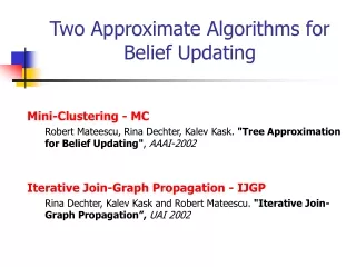
Two Approximate Algorithms for Belief Updating

Two Approximate Algorithms for Belief Updating Mini-Clustering - MC Robert Mateescu, Rina Dechter, Kalev Kask. "Tree Approximation for Belief Updating", AAAI-2002 Iterative Join-Graph Propagation - IJGP Rina Dechter, Kalev Kask and Robert Mateescu. "Iterative Join-Graph Propagation”, UAI 2002

What is Mini-Clustering? • Mini-Clustering (MC) is an approximate algorithm for belief updating in Bayesian networks • MC is an anytime version of join-tree clustering • MC applies message passing along a cluster tree • The complexity of MC is controlled by a user-adjustable parameter, the i-bound • Empirical evaluation shows that MC is a very effective algorithm, in many cases superior to other approximate schemes (IBP, Gibbs Sampling)

A B E C D F G Belief networks • The belief updating problem is the task of computing the posterior probability P(Y|e) of query nodes Y  X given evidence e.We focus on the basic case where Y is a single variable Xi

Cluster Tree Elimination • Cluster Tree Elimination (CTE) is an exact algorithm • It works by passing messages along a tree decomposition • Basic idea: • Each node sends only one message to each of its neighbors • Node u sends a message to its neighborvonly when ureceived messages from all its other neighbors

Cluster Tree Elimination • Previous work on tree clustering: • Lauritzen, Spiegelhalter - ‘88 (probabilities) • Jensen, Lauritzen, Olesen - ‘90 (probabilities) • Shenoy, Shafer - ‘90, Shenoy - ‘97 (general) • Dechter, Pearl - ‘89 (constraints) • Gottlob, Leone, Scarello - ‘00 (constraints)

Belief Propagation x1 h(u,v) v u x2 xn

A B E C D F G Cluster Tree Elimination - example ABC 1 BC BCDF 2 BF BEF 3 EF EFG 4

Cluster Tree Elimination - the messages A B C p(a), p(b|a), p(c|a,b) 1 BC B C D F p(d|b), p(f|c,d) h(1,2)(b,c) 2 sep(2,3)={B,F} elim(2,3)={C,D} BF B E F p(e|b,f), h(2,3)(b,f) 3 EF E F G p(g|e,f) 4

Cluster Tree Elimination - properties • Correctness and completeness: Algorithm CTE is correct, i.e. it computes the exact joint probability of a single variable and the evidence. • Time complexity: O ( deg  (n+N)  d w*+1 ) • Space complexity: O ( N  d sep) where deg = the maximum degree of a node n = number of variables (= number of CPTs) N = number of nodes in the tree decomposition d = the maximum domain size of a variable w* = the induced width sep = the separator size

Mini-Clustering - motivation • Time and space complexity of Cluster Tree Elimination depend on the induced width w* of the problem • When the induced width w* is big, CTE algorithm becomes infeasible

Mini-Clustering - the basic idea • Try to reduce the size of the cluster (the exponent); partition each cluster into mini-clusters with less variables • Accuracy parameter i = maximum number of variables in a mini-cluster • The idea was explored for variable elimination (Mini-Bucket)

Mini-Clustering • Suppose cluster(u) is partitioned into p mini-clusters: mc(1),…,mc(p), each containing at most i variables • TC computes the ‘exact’ message: • We want to process each fmc(k) f separately

Mini-Clustering • Approximate each fmc(k) f , k=2,…,p and take it outside the summation • How to process the mini-clusters to obtain approximations or bounds: • Process all mini-clusters by summation - this gives an upper bound on the joint probability • A tighter upper bound: process one mini-cluster by summation and the others by maximization • Can also use mean operator (average) - this gives an approximation of the joint probability

Idea of Mini-Clustering Split a cluster into mini-clusters =>bound complexity

Mini-Clustering - example ABC 1 BC BCDF 2 BF BEF 3 EF EFG 4

Mini-Clustering - the messages, i=3 A B C p(a), p(b|a), p(c|a,b) 1 BC B C D p(d|b), h(1,2)(b,c) C D F p(f|c,d) 2 sep(2,3)={B,F} elim(2,3)={C,D} BF B E F p(e|b,f), h1(2,3)(b), h2(2,3)(f) 3 EF E F G p(g|e,f) 4

Cluster Tree Elimination vs. Mini-Clustering ABC ABC 1 1 BC BC BCDF BCDF 2 2 BF BF BEF BEF 3 3 EF EF EFG 4 EFG 4

Mini-Clustering • Correctness and completeness: Algorithm MC(i) computes a bound (or an approximation) on the joint probability P(Xi,e) of each variable and each of its values. • Time & space complexity: O(n  hw*  d i) where hw* = maxu | {f | f  (u)  } |

Normalization • Algorithms for the belief updating problem compute, in general, the joint probability: • Computing the conditional probability: • is easy to do if exact algorithms can be applied • becomes an important issue for approximate algorithms

Normalization • MC can compute an (upper) bound on the joint P(Xi,e) • Deriving a bound on the conditional P(Xi|e) is not easy when the exact P(e) is not available • If a lower bound would be available, we could use:as an upper bound on the posterior • In our experiments we normalized the results and regarded them as approximations of the posterior P(Xi|e)

Experimental results • Algorithms: • Exact • IBP • Gibbs sampling (GS) • MC with normalization (approximate) • Networks (all variables are binary): • Coding networks • CPCS 54, 360, 422 • Grid networks (MxM) • Random noisy-OR networks • Random networks We tested MC with max and mean operators • Measures: • Normalized Hamming Distance (NHD) • BER (Bit Error Rate) • Absolute error • Relative error • Time

Random networks - Absolute error evidence=0 evidence=10

Coding networks - Bit Error Rate sigma=0.22 sigma=.51

Noisy-OR networks - Absolute error evidence=10 evidence=20

CPCS422 - Absolute error evidence=0 evidence=10

Grid 15x15 - 0 evidence

Conclusion • MC extends the partition based approximation from mini-buckets to general tree decompositions for the problem of belief updating • Empirical evaluation demonstrates its effectiveness and superiority (for certain types of problems, with respect to the measures considered) relative to other existing algorithms

Two Approximate Algorithms for Belief Updating