Download
1 / 133
1.33k likes | 1.75k Views
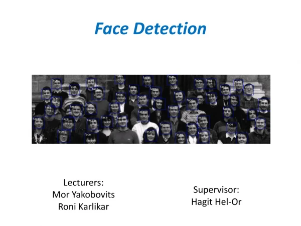
Face Detection. Lecturers: Mor Yakobovits Roni Karlikar. Supervisor: Hagit Hel-Or. Introduction. Humans can easily detect faces, although faces can be very different from each other. Humans have also tendency to see face patterns even if they don’t really exist. Faces everywhere.

E N D
Face Detection Lecturers: MorYakobovits RoniKarlikar Supervisor: Hagit Hel-Or
Introduction Humans can easily detect faces, although faces can be very different from each other.
Humans have also tendency to see face patterns even if they don’t really exist.
Faces everywhere http://www.marcofolio.net/imagedump/faces_everywhere_15_images_8_illusions.html
Face Detection • The problem of face detection is:Given an image, say if it contains faces or not. • The idea of face detection in computer vision is to let the computer learn to detect faces in images, just as a human can do.
Applications of Face Detection • Auto-focus in cameras • Security systems (recognize faces of certain people) • Human-computer interface • Marketing systems • Much more..
Difficulties of Face Detection Building a model for faces is not a simple task, faces can be complex and vary from each other. Faces in images are also affected from the environment.
Difficulties - Changing lightening • Affects color, facial feature
Difficulties - Skin Tone • Large variety of skin tones.
Difficulties - Facial Expressions • Affects shape of face and its features
Difficulties - Obstructions • Obstruction of facial features
Today’s Lecture • We will talk about: • Skin detection • Eigenfaces • Viola-Jones algorithm
Today’s Lecture • All of the 3 approaches we’ll see today are based on learning. • The computer learns to detect faces.
Learning - Intro • The learning model we’ll use is Classifier. • Purpose: classify data to several classes. • Training level: let the computer learn the features of each class (face & non-face). This is done using a dataset with examples for instances of each class. (the instances are already classified) • Classification: given a new instance, tell which class it belongs. Example: Studying for exam by solving previous exams.
Face Detection Using Skin Detection Probabilistic Approach image source
Skin Detection • Purpose: • Find “skin pixels” in a given image. • The main question: • How to determine if a pixel is a “skin pixel”? • Our approach will be to teach the computer what color is a skin color and what color isn’t.
Skin Detection • Skin detection is a color(pixel) – based approach for detecting faces. • This approach is quite simple • but has limited results due to • high sensitivity to illumination and other changes in skin tones • not only faces contain skin (arms, legs…) • some objects have similar colors to skin (for example, wooden furniture)
a yellow-biased face image (b) a light-compensated image (c) skin regions of (a) in white (d) skin regions of (b) Example for how illumination cause false-negative and false-positive detection. “Detecting Faces in Color Images” by Hsu, Abdel-Mottaleb & Jain
Another examples for false-positive (chair in top left corner) & false-negative (dark area of face in the image of the soccer player) skin detections. Rehg & Jones (1999)
Skin Colors In RGB Color Space 97% of the skin-color bins overlaps with non-skin color bins. explanation could be - many objects whose color resemble a skin color, like walls, railtracks, furnitures and wooden objects. Rehg & Jones (1999)
Skin Classifier • The problem: • Given a pixel x with color (r,g,b), determine if it’s a skin or not. skin
Skin Classifier • Given x = (R,G,B), how do we determine it’s class? (skin/non-skin) • Nearest neighbor • find labeled pixel closest to X • choose the class that pixel • Data modeling • fit a model (curve, surface, or volume) to each class • Probabilistic data modeling • fit a probability model to each class • we’ll focus on this approach Orange dots – skin Purple dots – non skin source
Probabilistic Skin Classifier • Two approaches we’ll discuss • Gaussian-Based (parametric model) • Histogram-Based (non-parametric model)
Parametric modeling Main Idea: • Assume the type/shape of the distribution we’re trying to find. • Find the parameters values for the assumed type from a training set.
Gaussian-Based Approach • (Parametric model) • Single Gaussian Model • We assume the probabilistic distribution we are trying to find is a Normal Distribution (Gaussian function) • To find that distribution, all we need is: • - mean of the learned skin colors • - covariance matrix of the learned skin colors is a color vector! Those parameters are evaluated separately for each class
Gaussian-Based Approach • (Parametric model) • After we have the mean & covariance, we get: • Where is the mean vector and is the covariance matrix of class j • For j=skin & j=non-skin
What we have • P(rgb / skin) & P(rgb / ~skin) – “probability that a (non-)skin pixel will have the color rgb” But that’s not what we want.
What we need • We need P(skin / rgb) & P(~skin / rgb) – “the probability that a pixel with the color rgb is (non-) skin” Remember Bayes’ Rule? After we achieve that, we can use MAP estimation.
Bayes’ Rule P(skin) is the portion of skin pixels from total pixels in the learning dataset P(R) can be calculated using the probabilities we already have.
MAP Estimation (Maximum A Posteriori estimation) Classification: A pixel with color R will be classified as skin iff P(skin / R) is higher than P(~skin / R) • MAP estimation- • Maximizes the probability for the posterior, and so • Minimizes the probability for false-negative misclassification • False-negative misclassification: a skin pixel classified as non-skin
Another Gaussian-Based Approach • (Parametric model) • Problem with Single Gaussian Model: • Actual skin distribution might be too complex to be represented as a Gaussian distribution. • Solution: Mixture of Gaussians (MoG) • Represent the distribution with several different Gaussian distributions to allow more dynamic modeling of the distribution
Skin Color distribution in HSV color space • HSV (Hue, Saturation, Value) • separates color components from intensity • (in RGB intensity affects all channels) • - Not the best color space for color-based approaches, but conversion is very simple compared to the better color spaces source
Gaussian-Based Approach • (Parametric model) • Drawback: • Slower learning because we need to use EM algorithm to estimate the MoG • Slower classification, since it requires a evaluation all of the Gaussians • In the case of Mixture of Gaussians: Classification: Use Bayes’ and then MAP
MoG vs. Single Gaussian Single Gaussian Training set distribution MoG source
Non-parametric modeling Main Idea: • Do not assume anything about the distribution we are looking for. • Derive the distribution directly from the dataset.
Histogram-Based Approach • Non-parametric model • Learn from a labeled dataset • for each color bin (256*256*256 ~ 16.7m in RGB), count • how many pixels of that color were skin • how many pixels of that color were non-skin • We get a histogram: (Our histograms will have three dimensions) And a equivalent histogram for non-skin pixels.
Histogram-Based Approach • Non-parametric model • we have P(rgb / skin) & P(rgb / ~skin) • we need P(skin / rgb) & P(~skin / rgb)
Histogram-Based Approach • Non-parametric model • A 3D histogram looks like this: • Viewing direction along the green-magenta axis which joins corners (0,255,0) and (255,0,255) in RGB • The viewpoint was chosen to orient the gray line horizontally • 8 bins in each color channel • Only shows bins with counts greater than 336,818 Rehg & Jones (1999)
Histogram-Based Approach • Non-parametric model • Step by step explanation: • Learning: • Using a labeled dataset: • For each color X: count how many occurrences of X as skin pixel & non-skin pixels: • Normalize each histogram for each color X: & respectively
Histogram-Based Approach • Non-parametric model • Step by step explanation: (cont’d) • Learning: 3. Apply bayes’ rule, for each color X: • We have P(X|skin) from histogram N • .P(skin) = • . • P(X) = • Symmetrically for
Histogram-Based Approach • Non-parametric model • Step by step explanation: (cont’d) • Classification: • We are given a color X • Determine class with: (MAP estimation) • Only 2 table look-ups! • One in the skin histogram and one in the non-skin histogram
Histogram-Based Approach - Example • Non-parametric model • Assume we observed from the dataset: • 534 skin-pixels with the color (100, 100, 100) • 330 non-skin pixels with the color (100, 100, 100) • Total number of observed pixels is 10000 • 5000 skin pixels • 5000 non-skin pixels • We get the corresponding probabilities: • P((100, 100, 100)| Skin ) = 534/5000= 0.1068 • P((100, 100, 100)| Non-skin ) = 330/5000= 0.066 • The histograms (skin & non-skin):
Example – cont’d Reminder: Bayes’ Rule - • P((100, 100, 100)| Skin ) = 0.1068 • P((100, 100, 100)| ~Skin ) = 0.066 • Using Bayes’ Rule: • P((100, 100, 100) | Skin ) is bigger than P((100, 100, 100) | ~Skin ) • And so every pixelwith the color(100, 100, 100) will be classified as a skin pixel
Bibliography • Statistical Color Models with Application to Skin Detection by Rehg & Jones (1999) • “Detecting Faces in Color Images” by Hsu, Abdel-Mottaleb & Jain (2002) • “A Survey on Pixel-Based Skin Color Detection Techniques” byVezhnevets, Sazonov & Andreeva (2003) • http://alumni.media.mit.edu/~maov/classes/comp_photo_vision08f/lect/05_skin_detection.pdf • http://pages.cs.wisc.edu/~lizhang/courses/cs766-2007f/syllabus/10-23-recognition/10-22-recognition.ppt
Eigenfaces M.A. Turk and A.P. Pentland: Eigenfaces for Recognition. Journal of Cognitive Neuroscience, 3 (1):71--86, 1991.