Download
1 / 23
230 likes | 307 Views
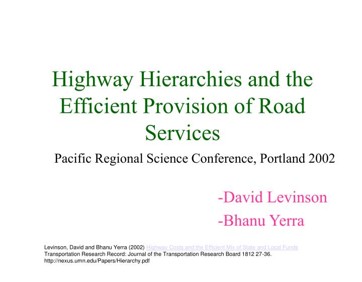
Highway Hierarchies and the Efficient Provision of Road Services. Pacific Regional Science Conference, Portland 2002. -David Levinson -Bhanu Yerra. Levinson, David and Bhanu Yerra (2002) Highway Costs and the Efficient Mix of State and Local Funds

E N D
Highway Hierarchies and the Efficient Provision of Road Services Pacific Regional Science Conference, Portland 2002 -David Levinson -Bhanu Yerra Levinson, David and Bhanu Yerra (2002) Highway Costs and the Efficient Mix of State and Local Funds Transportation Research Record: Journal of the Transportation Research Board 1812 27-36. http://nexus.umn.edu/Papers/Hierarchy.pdf
Introduction • Hierarchies in Highways and Governments • Government layers responsible for a Highway class • Scale Economies?
Figure 1: Functional Highway Classification and Type of Service Provided
Interstate Arterials Collectors Local Streets Federal Others State Operation Local Capital Government Costs Theory • A third dimension to the problem - Costs Figure 2: Schematic representation of three dimensional structure of highways, costs and government layers
Cost spent on a highway class Minimum Cost State Share of expenditure 100% 0% Optimal expenditure share Figure 3: Parabolic variation of cost with respect to state's expenditure share Theory Contd. • Parabolic variation of Cost with Expenditure share by state government
Table 1: Top five states financed by Local Government Theory Contd. • Existing Expenditure Structure
Table 2: Top five states financed by State Government Theory Contd.
Data • Variables considered in this study • Cost variables • Expenditures- Capital Outlay, Maintenance and Total Expenditure per year in a state • Expenditure Share • Network variables • Length of highways in a state • Output variables • Vehicle miles traveled (VMT) by Passenger cars • Vehicle miles traveled (VMT) by trucks
Data Contd. • Instrumental Variables (IV) • Necessity of IV model • Percentage of VMT by a vehicle type is not available for lower highway classes • Issues in formulating IV model • Model generalized for all roadway classes • Rank of a roadway class as a variable • Zipf’s law • Model generalized for all states
Data Contd. • IV Model • i represents state, • j represents highway class, j - 1 .. 12, • is the estimated % of VMT by the passenger cars in ith state on jth highway class, • is the estimated % of VMT by the trucks in ith state on jth highway class, • Rj represents the rank of the jth class of highway, • vij represents the % of total VMT in jth class of highway, in ith state, • lij represents the % of road length of jth roadway class in ith state, • 's, 's, 's, 's are coefficients from the regression
Data Contd. • Results
Data Contd. • Calculating output variables using IV model • pi represents millions of VMT by passenger cars in ith state, • ti represents millions of VMT by trucks in ith state, • Vj is total vehicle miles traveled by all vehicle types on the jth class of roads.
Model • Cost variables Table 4: Table explaining the relationship between cost variables
Model Contd. • Cost variables Contd. • e is total cost of capital outlay and maintenance, • c is capital outlay cost, • m is maintenance cost, • es is total cost financed by state and federal government, • el is total cost financed by local government, • cs is capital outlay financed by state and federal government, • cl is capital outlay financed by local government, • ms is maintenance cost financed by state and federal government, • ml is maintenance cost financed by the local government.
Model Contd. • Expenditure share variables • qs,e is expenditure share of total cost by state and federal government, • qs,c is expenditure share of capital outlay by state and federal government, • qs,m is expenditure share of maintenance costs by state and federal government.
Model Contd. • Cost functions • l is length of highways in a state in thousands of miles, • p is millions of vehicle miles traveled by passenger cars in a state, • t is millions of vehicle miles traveled by trucks in a state. • Why Square of expenditure share by state a variable in the model?
Model Contd. • Quasi Cobb-Douglas function • a’s and b’s are regression coefficients • Only two regression functions since the degrees of freedom of the problem is 4
Model Contd. • Why variables (p/l) and (t/p+t) are used? • Multicollinearity • Cost functions has an optimal expenditure share (convex function) if and only if for total expenditure function for capital outlay function
Results Table 5: Regression results for Total expenditure
Table 6: Regression results for Capital Outlay Results Contd.
Results Contd. • Optimal Expenditure share qs,e,min is the optimal total expenditure share by state qs,c,min is the optimal capital outlay share by state Table 7: Table showing optimal vales and 95% confidence interval for state expenditure share
Results Contd. • Marginal and Average Costs Table 8: Marginal and Average costs for Total Expenditure and Capital Outlay
Conclusion and Recommendations • Parabolic nature of cost functions • Most of the states are within the 95% confidence interval of optimal expenditure share of capital outlay • Most of the states are out of the 95% confidence interval of optimal expenditure share of Total expenditure • All states together can save $10 billion if all of them are at optimal point. • Financial policies