Download
1 / 36
360 likes | 369 Views
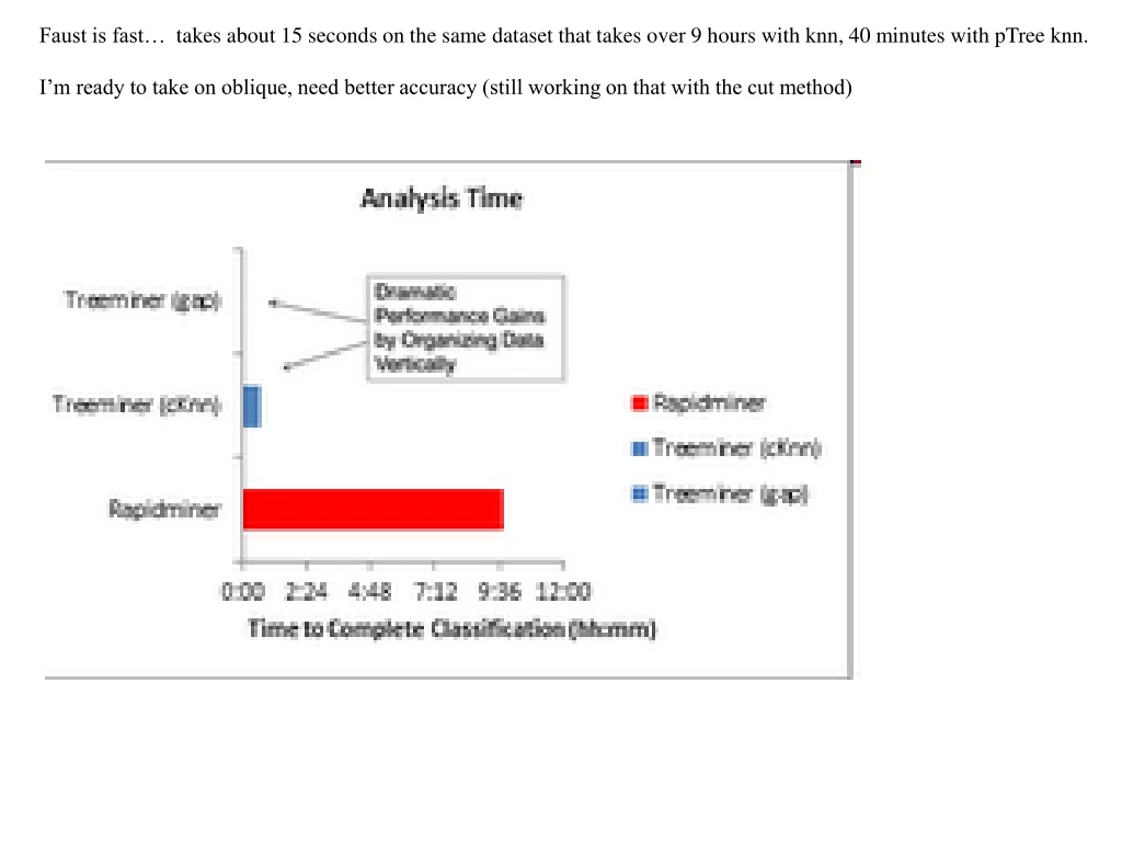
Faust is fast… takes about 15 seconds on the same dataset that takes over 9 hours with knn, 40 minutes with pTree knn. I’m ready to take on oblique, need better accuracy (still working on that with the cut method).

E N D
Faust is fast… takes about 15 seconds on the same dataset that takes over 9 hours with knn, 40 minutes with pTree knn. I’m ready to take on oblique, need better accuracy (still working on that with the cut method)
Some data. I started doing some experiments on faust to assess cutting off classification when gaps got too small (with an eye towards using knn or something from there). Results are pretty darn good if you ask me… and for faust this is still single gap, working on total gap (maximum of (minimum of prev and next gaps)) Here’s also a new data sheet I’ve been working on focused on gov’t clients -Mark
From: Keith Murphy [mailto:kmurph2@clemson.edu] Sent: Tuesday, March 06, 2012 5:30 PMTo: Perrizo, Willia Yes, pTREES for med informatics, Bill!!!! You and I and your team could work so many miracles..... the data we can generate requires robust informatics and comp. biology. I would put resources into this I am so excited to be here this week. CONGRATS ON YOUR AWARDS. Goodness, we need to move..... K Keith E. Murphy, Ph.D. Professor and ChairDepartment of Genetics and Biochemistry Director, Clemson University Genomics InstituteClemson University Clemson, SC 29634-0318 • From: Perrizo, William [William.Perrizo@ndsu.edu] Sent: Tuesday, March 06, 2012 6:27 PM To: Keith Murphy Hi Keith, I forgot to point out in the slides that we have applied pTrees to Bioinformatics successfully too (took second in the 2002 ACM KDD-cup in bioinformaticsand took first in the 2006 ACM KDD-cup in medical informatics. 2006 Association of Computing Machinery (ACM) Knowledge Discovery and Data Mining (KDD) Cup Winning Team Leader Task 3. Negative Prediction of Computer Aided Detection (CAD) of Pulmonary Embolism from Computer Aided Tomography (CAT) data. (Our team score was twice as high as the next closest competitor score ), see http://www.cs.unm.edu/kdd_cup_2006, http://www.cs.unm.edu/files/kdd-cup-2006-task-spec-final.pdf . The following description was lifted from these pages: 2002 Assoc of Comp Machinery (ACM) Knowledge Discovery and Data Mining (KDD) Cup, Task 2. Yeast Gene Regulation Prediction: There are now experimental methods that allow biologists to measure some aspect of cellular "activity" for thousands of genes or proteins at time A key problem that often arises in such experiments is in interpreting or annotating these thousands of measurements. This KDD Cup task focused on using data mining methods to capture the regularities of genes that are characterized by similar activity in a given high-throughput experiment. To facilitate objective evaluation, this task did not involve experiment interpretation or annotation directly, but instead it involved devising models that, when trained to classify the measurements of some instances (i.e. genes), can accurately predict the response of held aside test instances. The training and test data came from recent experiments with a set of S. cerevisiae (yeast) strains in which each strain is characterized by a single gene being knocked out. Each instance in the data set represents a single gene, and the target value for an instance is a discretized measurement of how active some (hidden) system in the cell is when this gene is knocked out. The goal of the task is to learn a model that can accurately predict these discretized values. Such a model would be helpful in understanding how various genes are related to the hidden sys See http://www.acm.org/sigs/sigkdd/kddcup/index.php?section=2002&method=res
Commodity trading room in Barry Hall nears completion A new space for students to learn about commodity marketing, logistics, trading and risk management is nearing completion in Richard H. Barry Hall. The commodity trading room is scheduled to be available for classes starting next fall. Equipment installation is planned for June. William Wilson, University Distinguished Professor, said in a media release, the room was developed in response to the growth in commodities trading and the importance of commodity trading to North Dakota, which includes trading in agricultural, energy and transportation products. “The output will be more and better trained students who will work in the different segments of these industries,” he said. Wilson said the trading room should be viewed as a laboratory for analyzing markets and financial instruments, no different than a laboratory for biology or chemistry. Students will have the ability to analyze portfolios, trading strategies and risks. “All of these are important in North Dakota and the region,” Wilson said. “Most competing business schools have financial and trading rooms. Developing a trading room in Barry Hall will provide similar training and research opportunities for NDSU students and faculty. For the agribusiness industry, NDSU will be the first school having such capabilities that focus on agriculture and the biofuels sector.” The room is modeled after a similar project at Tulane University, New Orleans. Technically, it will have 32 work stations. Sixteen of the work stations will have access to live commodity and financial market information for agriculture, commodities and financials. The number of live stations will be expanded in the future. The trading room will be used for teaching courses in agribusiness and the College of Business. Opportunities also will be explored through the Tri-College University system. There are plans to develop numerous outreach programs for individual firms, commodity organizations, Northern Crops Institute, biofuels sector and fee-based advanced programs. Funding for the commodity trading room has been provided by the North Dakota Agricultural Experiment Station, vice president for academic affairs and NDSU Technology Fee Advisory Committee. The funds are seed money for computers and other hardware. Wilson said the project has been encouraged by major agribusiness firms that have provided varying forms of financial support, including ADM, CHS, Gavilon, The Rice Trader and George M. Schuler III of Minn-Kota Ag Products Inc. A number of state commodity organizations also have provided funding, including the North Dakota Corn Council, North Dakota Soybean Council, North Dakota Wheat Commission and Northern Crops Institute. He said other agribusiness firms and entities have expressed interest in a sponsorship. The NDSU Development Foundation is working toward establishing an endowment for the permanent support of the commodity trading room.
Two new Centers of Research Excellence at NDSU approved The North Dakota Centers of Excellence Commission has approved $1.67 million to fund two new Centers of Research Excellence at NDSU. NDSU will receive $1.35 million to develop a new Center of Research Excellence called the Center for Life Sciences Research and Applications, which will conduct life sciences research with private partners, including Sanford Research and the RJ Lee Group Inc. The commission also approved $320,000 to establish the Center for Technologically Innovative Products and Processes. Initially, this center will partner with industrial companies such as Mid-America Aviation, Amity Technology and Arkema Inc., assisting with product research, testing, evaluation and analysis. “These research centers are promising economic development projects for the state of North Dakota,” North Dakota Commerce Commissioner Al Anderson said. “Centers of Research Excellence projects help us leverage the talent and research expertise that exists in our state.”
NDSU Center for Life Sciences Research and Applications (NDSU will receive $1.35 million to develop from state centers of excellence) Sanford Research, headquartered in Sioux Falls, S.D., and Fargo, plans to partner with the new Center for Life Sciences Research and Applications for research on human genomics and bioinformatics. Initial focus is expected to include breast cancer research and research into certain rare diseases in children. Sanford Research and RJ Lee have committed to contribute cash and in-kind contributions totaling $2.7 million to the center during a period of more than four years. “Sanford Research is pleased to partner with NDSU in this important health research initiative,” said Ruth Krystopolski, executive vice president of development and research at Sanford Health. “We share the belief in and enthusiasm for the application of genomic information toward novel clinical trials, next-generation therapies and cures. Already, advances in clinical genomics have enhanced translational research activities in type 1 diabetes, breast cancer and childhood rare diseases among other disciplines at Sanford Research. This project will allow for an even greater level of integration between scientific discovery and the doctor’s office, and most importantly, improve care for the patients we serve in our region.” In addition, the RJ Lee Group Inc., a major supplier of industrial forensic capabilities, plans to work with the center and the NDSU DNA Laboratory to develop next generation DNA-based identification and forensic tests and methods. Based in Monroeville, Penn., the group was founded by North Dakota native Richard J. Lee. The goal of the center is to combine the resources and capabilities of multiple private sector partners interested in the life sciences with NDSU’s research and development capabilities for life science-related technology or product development. “These centers will be a significant addition to NDSU’s research efforts benefiting our state’s economy, while leading to opportunities for students, both in their studies and in their future careers. The centers provide technology-based economic stimulation that only can come from the comingling of research university and business development activities,” said NDSU President Dean L. Bresciani. “NDSU’s involvement in these exceptional research partnerships will involve graduate and undergraduate students participating in research activities by the center and its partners. In parallel with this CORE effort, NDSU also plans to offer additional opportunities for postgraduate studies and research in genetics and bioinformatics,” said Bruce Rafert, NDSU provost. “This new center builds upon NDSU’s expertise in robotics, computational sciences and informatics. It can also serve as another catalyst in the burgeoning life sciences industry cluster in the Red River Valley, further contributing to technology-based economic development,” said Philip Boudjouk, vice president for research at NDSU. The center will initially focus on discoveries and technologies generated by NDSU and private sector partners that have the potential to: • Encourage growth of the life sciences industry sector in North Dakota and promote technology-based economic development, • Spur growth of computational research and sciences, particularly in bioinformatics, • Spur growth of genomics research, and • Spur growth of DNA-based forensics and identification research and applications. Genomics involves studying the function and interactions of all genes in the genome. Such research can involve humans, plants or animals. In human genomics, researchers use biological roadmaps to find which genes might be involved in diseases such as cancer. In plants, it might be which genes play a role in crop disease and performance. In animals, genomics research can lead to a better understanding of disease resistance and susceptibility. Bioinformatics uses computational technologies to manage and analyze vast amount of research info that is generated. Computer technology can be used to uncover info hidden in large masses of data, helping to better diagnose and treat diseases in humans, plants and animals.
NDSU Center for Technologically Innovative Products and Processes The center stems from requests from private sector partners of existing NDSU Centers of Excellence to engage in commercially relevant research projects involving the entire product supply chain, including material design and selection, researching process improvements, testing and evaluating product prototypes, analyzing product failure, and research to improve products. The center will focus on market-driven research to enhance products, reduce production costs and improve processes. Center partners will utilize NDSU’s expertise in such areas as materials characterization, corrosion research, chemistry and engineering. Another goal of the program is to promote the use of technological developments that have a cost effective, but positive environmental effect in the energy industrial cluster in the western part of the state. Initial partners include Mid-America Aviation, a leader in the aerospace industry based in West Fargo; Amity Technology, a leader in agricultural equipment applications, in Fargo; and Arkema Inc., a global producer of industrial chemicals, performance products and vinyl products, based in King of Prussia, Pa., that is developing products to better serve the needs of wind-based energy production, a growing energy segment in North Dakota. The three initial private sector partners have committed cash and in-kind match contributions totaling $640,000 for the new research center. “The Center of Research Excellence program will provide substantial benefit to Mid-America Aviation by enabling us to leverage the great facilities and personnel at North Dakota State University to provide research support for our development of new overhaul and manufacturing technologies,” said Randall D. Herman, chief operating officer, Mid-America Aviation. “This partnership with the state of North Dakota, NDSU and Mid-America Aviation represents the best possible utilization of public and private resources to enhance business opportunities in our region, to grow our business and to provide better employment opportunities to our workforce.” The center also will enable NDSU students to participate in industrially relevant research. “It will conduct commercially-relevant research driven by the market, helping companies solve product supply chain problems, while giving students substantial research experience in this business sector,” Boudjouk said. The center will work with industrial partners from the beginning of the industrial supply chain through to finished products.
Multi-hop Data Mining (MDM): relationship1 (e.g., Buys= B(P,I) ties table1 Category color size wt store city state country P=People, I=Items, F(P,C)=Friends, B(C,I)=Buys Find all strong, AC, AP, CI frequent iff ct(PA)>minsup and confident iff ct(&pAPpAND &iCPi) > minconf ct(&pAPp) This says: "a friend of all in A will buy C if all in A buy C." (note the AND is always AND) closures: A freq then A+ freq. AC not conf, then AC- not conf 2 2 3 3 4 4 5 5 P 2 3 0 1 1 0 0 1 0 1 1 0 0 0 1 0 0 1 4 5 ct(|pAPpAND &iCPi) >mncnf ct(|pAPp) ct(|pAPpAND |iCPi) >mncnf ct(|pAPp) Change to "a friend of any in A will buy C if any in A buy C. Change to "a friend of any in A will buy something in C if any in A buy C. pc bc lc cc pe age ht wt (e.g., People=P=an axis with descriptive features columns) to table_2 (e.g., Items). Table_2 (I=Items) is tied by relationship_2 (e.g., Friends=F(P,P) ) to table_3 (e.g., also P)... Can we do interesting clustering and/or classification on one of the tables using the relationships to define "close" or to define the other notions? I=Items F(P,P)=Friends 0 0 0 1 0 1 0 0 0 0 0 0 0 0 1 0 B(P,I)=Buys P=People Define the NearestNeighbor VoterSet of {f} using strong R-rules with F in the consequent? A correlation is a relationship A strong cluster based on several self-relationships (but different relationships, so it's not just strong implication both ways) is a set that strongly implies itself (or strongly implies itself after several hops (or when closing a loop).
1 0 0 0 1 0 0 bpp 1 2 3 4 5 ... 3B 0 1 1 0 0 1 1 0 0 0 0 0 0 0 1 0 0 0 1 0 0 1 1 2 2 0 0 1 0 0 0 1 3 3 1 0 0 0 1 0 0 4 4 0 0 1 0 0 0 0 5 5 AHG(P,bpp) ... ... 7B 7B P P gene chromosome bpp 1 2 3 4 5 ... 3B pc bc lc cc pe age ht wt 1 0 0 0 1 0 0 0 1 1 0 0 1 1 0 0 0 0 0 0 0 1 0 0 0 1 0 0 0 0 1 0 0 0 1 1 0 0 0 1 0 0 0 0 1 0 0 0 0 AHG(P,bpp) Bioinformatics Data Mining: Most bioinformatics done so far is not really data mining but is more toward the database querying side. (e.g., a BLAST search). What would be real Bioinformatics Data Mining (BDM)? A radical approach View whole Human Genome as 4 binary relationships between People and base-pair-positions (ordered by chromosome first, then gene region?). AHG is the relationship between People and adenine (A) (1/0 for yes/no) THG is the relationship between People and thymine (T) (1/0 for yes/no) GHG is the relationship between People and guanine (G) (1/0 for yes/no) CHG is the relationship between People and cytosine (C) (1/0 for yes/no) Order bpp? By chromosome and by gene or region (level2 is chromosome, level1 is gene within chromosome.) Do it to facilitate cross-organism bioinformatics data mining? This is a comprehensive view of the human genome (plus other genomes). Create both a People-PTreeSet and bpp PTreeSet vertical human genome DB with a human health records feature table associated with the people entity. Then use that as a training set for both classification and multi-hop ARM. A challenge would be to use some comprehensive decomposition (ordering of bpps) so that cross species genomic data mining would be facilitated. On the other hand, if we have separate PTreeSets for each chrmomsome (or even each regioin - gene, intron exon...) then we can may be able to dataming horizontally across the all of these vertical pTree databases. The red person features used to define classes. AHGp pTrees for data mining. We can look for similarity (near neighbors) in a particular chromosome, a particular gene sequence, of overall or anything else.
Facebook-Buys example I≡Items F≡Friends(M,M) Members 1 0 1 1 4 0 1 0 0 3 1 0 0 1 2 0 0 1 0 1 P≡Purchase(M,I) 4 2 3 3 2 4 5 1 Members 2 0 1 0 1 1 0 1 1 1 1 0 1 0 1 1 1 1 1 0 0 1 4 3 2 1 4 0 1 1 0 1 1 2 0 A facebook Member, m, purchases Item, x, tells all friends. Let's make everyone a friend of him/her self. Each friend responds back with the Items, y, she/he bought and liked. K2 = {1,2,4} P2 = {2,4} ct(K2) = 3 ct(K2&P2)/ct(K2) = 2/3 XI MX≡&xXPx People that purchased everything in X. FX≡ORmMXFb = Friends of a MX person. So, X={x}, is Mx Purchases x strong" Mx=ORmPxFm x frequent if Mx large. This is a tractable calculation. Take one x at a time and do the OR. Mx=ORmPxFm x consequent if Mx large. ct( Mx Px ) / ct(Mx) > minconf ct( ORmPxFm & Px ) / ct( ORmPxFm ) > minconf To mine through all X, we start with X={x}. If not confident then no superset will be either. Therefore we have closure and can only consider X={x.y} for x and y forming confident rules themselves....
Examples I≡Items F≡Friends(K,B) Buddies 1 0 1 1 4 0 1 0 0 3 1 0 0 1 2 0 0 1 0 1 P≡Purchase(B,I) Kiddos 4 2 3 3 4 2 5 1 Groupies 4 1 0 1 1 4 4 2 2 1 3 0 1 0 0 3 2 1 0 0 1 2 1 0 0 1 0 1 1 1 0 1 1 1 1 1 0 1 1 1 1 0 1 1 0 0 1 4 3 2 1 4 0 0 1 0 1 1 0 0 0 Others(G,K) 1 1 1 1 1 0 1 1 2 1 0 1 0 Assume a facebook buddy, b, purchases x, tells all friends. Let's make everyone a buddy of himself or herself. Each friend tells all their friends. We advertise to those friends of friends.: K2 = {1,2,3,4} P2 = {2,4} ct(K2) = 4 ct(K2&P2)/ct(K2) = 2/4 Kx=OR Og x frequent if Kx large. This is a tractable calculation. Take one x at a time and do the OR. gORbPxFb
Examples I≡Items F≡Friends(K,B) Buddies 1 0 1 1 4 0 1 0 0 3 1 0 0 1 2 0 0 1 0 1 P≡Purchase(B,I) Kiddos 4 2 3 3 4 2 1 5 Groupies 4 1 0 1 1 4 1 4 2 3 0 1 0 0 3 2 1 0 0 1 2 1 0 1 0 1 1 1 0 1 1 0 1 1 0 1 1 1 1 1 1 1 0 0 1 4 3 2 1 4 0 0 1 0 1 0 0 0 Compatriots (G,K) 1 1 1 1 0 1 1 2 0 0 1 Assume a facebook buddy, b, purchases x, tells all friends. Let's make everyone a buddy of himself or herself. Each friend tells all their friends. But we are interested in strong purchase possibilities. So we intersect rather than union (AND rather than OR). We advertise to those friends of friends.: K2 = {2,4} P2 = {2,4} ct(K2) = 2 ct(K2&P2)/ct(K2) = 2/2 The questions are: We are talking speed here (the same algorithms could be used in the horizontal data setting.) Are we faster? Note that unless the horizontal renditions of the relationship data are duplicated in dual form (all of them) they cannot possibly compete and even then they have to retrieve entire records twice (both duals).
Multi-level pTrees for data tables: Given a IRIS Table NameSLSWPLPWColor setosa 38 38 14 2 red setosa 50 38 15 2 blue setosa 50 34 16 2 red setosa 48 42 15 2 white setosa 50 34 12 2 blue versicolor 51 24 45 15 red versicolor 56 30 45 14 red versicolor 57 28 32 14 white versicolor 54 26 45 13 blue versicolor 57 30 42 12 white virginica 73 29 58 17 white virginica 64 26 51 22 red virginica 72 28 49 16 blue virginica 74 30 48 22 red virginica 67 26 50 19 red
Multi-level pTrees for data tables: Given a n-row table, a row predicate (e.g., a bit slice predicate, or a category map) and a row ordering (e.g., ascending on the key or, for spatial data, column/row-raster, Z=Peano or Hilbert), the sequence of predicate truth bits (1/0) is the raw or level-0predicate map (pMap) for that table, predicate and row order. gte50% str=5 pMC=red 0 0 1 pure1 str=5 pMC=red 0 0 0 gte25% str=5 pMC=red 1 1 1 pred: rem(div(SL/2)/2)=1 order: given order gte50% stride=5 pMSL,1 1 0 0 pure1 str=5 pMSL,1 0 0 0 gte25% str=5 pMSL,1 1 1 1 gte75% str=5 pMSL,1 1 0 0 IRIS Table NameSLSWPLPWColor setosa 38 38 14 2 red setosa 50 38 15 2 blue setosa 50 34 16 2 red setosa 48 42 15 2 white setosa 50 34 12 2 blue versicolor 51 24 45 15 red versicolor 56 30 45 14 red versicolor 57 28 32 14 white versicolor 54 26 45 13 blue versicolor 57 30 42 12 white virginica 73 29 58 17 white virginica 64 26 51 22 red virginica 72 28 49 16 blue virginica 74 30 48 22 red virginica 67 26 50 19 red pMSL,0 0 0 0 0 0 1 0 1 1 1 1 0 0 0 1 pMColor=red 1 0 1 0 0 1 1 0 0 0 0 1 0 1 1 pMSL,1 1 1 1 0 1 1 0 0 1 0 0 0 0 1 1 gte75% str=5 pMC=red 0 0 1 predicate: remainder(SL/2)=1 order: the given table order pred: Color='red' order: given ord gte50% stride=5 pMPW<7 1 0 0 pred: PW<7 order: given pMPW<7 1 1 1 1 1 0 0 0 0 0 0 0 0 0 0 Note the potential classification power of this gte50% stride=5 pMap-perfectly predicts setosa. Given a raw pMap, pM, a decomposition of it into mutually exclusive, collectively exhaustive bit intervals and a bit-interval-predicate, bip (e.g., pure1, pure0, gte50%Ones), the bip stride=m level-1 pMap of pM is the string of bip truth values generated by applying bip to the consecutive intervals of the decomposition When the decomposition is equiwidth, the interval sequences is fully determined by the width=m>1, AKA, stride=m pM and all of its level-1 pMaps constitute the pTree of the same name as pM
All non-raw pMaps are level-1 pMaps. If the intervals of one set of level-1 pMaps are subsets of another sets of pMaps, then the raw pMap together with all the level-1 pMaps can be viewed as a multi-level pTree: 0 1 1 1 1 0 0 1 0 0 level-2 gte50% stride=2 1 1 pMgte50%,s=4,SL,0 0 1 1 1 level-1 gt50 stride=4 pMap level-1 gt50 stride=2 pMap Level-2 pMaps? pred: rem(SL/2)=1 ord: given order gte50% stride=8 pMSL,0 0 1 gte50% stride=4 pMSL,0 0 1 1 1 gte50% stride=16 pMSL,0 0 IRIS Table 2 NameSLSWPLPWColor setosa 38 38 14 2 red setosa 50 38 15 2 blue setosa 50 34 16 2 red setosa 48 42 15 2 white setosa 50 34 12 2 blue versicolor 51 24 45 15 red versicolor 56 30 45 14 red versicolor 57 28 32 14 white versicolor 54 26 45 13 blue versicolor 57 30 42 12 white virginica 73 29 58 17 white virginica 64 26 51 22 red virginica 72 28 49 16 blue virginica 74 30 48 22 red virginica 67 26 50 19 red virginica 71 25 50 20 white pMSL,0 0 0 0 0 0 1 0 1 1 1 1 0 0 0 1 1 pMgte50%,s=4,SL,0≡ gte50% stride=4 pMSL,0 0 1 1 1 R11 1 0 0 0 1 0 1 1 pred: rem(SL/2)=1 ord: given order pMSL,0 0 0 0 0 0 1 0 1 1 1 1 0 0 0 1 1 raw level-0 pMap gte50_pTrees11 1 We define a level-2 pMap as one that is a level-1 pMap built on another level-1 pMap (considered to be a one-col table). level-2 pMaps has less utility than level-1's? (bit strings different). gte50%; es=4,8,16; \SL,0 pTree, denoted pTgte50%_s=4,8,16_SL,0
gte50 Satlog-Landsat stride=320, classes: 1=redsoil 2=cotton 3=greysoil 4=dampgreysoil 5=stubble 7=verydampgreysoil The table is: R G ir1 ir2 class WL band [w1,w2) 1 w1 w1 w2 w2 [w2,w3) 2 ... [w3,w4) ... ... w5000 w5000 [w4,w5) 4436 WLs WLs WLs pixels 21 43 110 160 3 18 21 21 21 21 43 43 43 43 110 110 110 110 202 14 0 160 160 160 160 3 3 3 3 18 18 18 18 29 152 230 202 202 202 202 14 14 14 14 0 0 0 0 10 10 10 10 1 10 1 29 29 29 29 152 152 152 152 230 230 230 230 78 78 78 4 78 78 4 155 155 7 155 155 155 7 54 54 2 54 2 54 54 class 1 1 w1 1 1 1 2 2 2 w2 2 2 ... ... ... ... ... ... 4436 4436 4436 4436 w5000 4436 pixels pixels WLs pixels pixels pixels and it generates the [labeled by value] relationships: Given a relationship, it generates two dual tables:
gte50 Satlog-Landsat stride=64, classes: redsoil cotton greysoil dampgreysoil stubble verydampgreysoil 320-bit strides start end cls cls 320 stride 2 1073 1 1 2 321 1074 1552 2 1 322 641 1553 2513 3 1 642 961 2514 2928 4 2 1074 1393 2929 3398 5 3 1553 1872 3399 4435 _7 3 1873 2192 4436 3 2193 2512 4 2514 2833 5 2929 3248 7 3399 3718 7 3719 4038 7 4039 4358 0 0 0 0 0 0 1 2 1 1 1 1 ... ... ... ... ... ... 255 255 255 255 255 255 r r r r c c c c g g g g d d d d s s s s v v v v cl cl cl cl 1 1 1 1 0 0 0 0 0 0 0 0 0 0 0 0 0 0 0 0 0 0 0 0 0 0 0 0 0 0 0 0 0 0 0 0 1 0 0 1 1 0 0 0 0 0 0 1 0 0 0 0 0 0 0 0 0 0 0 0 1 1 0 0 1 0 1 0 0 0 0 0 0 0 0 0 0 0 0 0 0 0 0 0 0 0 0 0 0 0 0 0 0 0 0 0 Rclass ir1class ir2class Gclass ir2 ir2 ir1 G ir2 ir1 0 0 0 0 0 0 0 1 0 0 0 0 0 0 0 0 0 0 0 0 0 0 0 0 0 0 1 0 0 0 0 0 0 0 1 1 1 1 1 1 1 1 1 1 0 0 0 0 0 1 0 0 0 0 0 0 0 0 0 0 0 1 1 0 0 0 0 0 R G ir1 ir2 cls means stds means stds means stds means stds 1 64.33 6.80 104.33 3.77 112.67 0.94 100.00 16.31 2 46.00 0.00 35.00 0.00 98.00 0.00 66.00 0.00 3 89.33 1.89 101.67 3.77 101.33 3.77 85.33 3.77 4 78.00 0.00 91.00 0.00 96.00 0.00 78.00 0.00 5 57.00 0.00 53.00 0.00 66.00 0.00 57.00 0.00 7 67.67 1.70 76.33 1.89 74.00 0.00 67.67 1.70 ... ... ... ... ... ... ... ... ... ... 1 1 0 1 0 0 1 0 1 0 0 0 1 0 1 1 0 0 0 1 1 0 0 0 255 255 255 255 255 255 255 255 255 255 1 0 0 0 0 1 0 0 1 0 1 1 0 0 0 0 1 0 0 0 0 0 1 0 R ir1 R R ir2 G G G ir1 R Rir2 Gir2 ir1ir2 Rir1 RG Gir1 For gte50 Satlog-Landsat stride=320, we get: Note that for stride=320, the means are way off and it therefore will probably produce very inaccurate classification.. A level-0 pVector is a bit string with 1 bit per record. A level-1 pVector is a bit string with 1 bit per record stride which gives truth of a predicate applied to record stride. A n-level pTree consists of a level-k pVector (k=0...n-1) all with the same predicate and s.t. each level-k stride is a contained within one level-k-1 stride.
R 1 2 3 4 5 7 cls 14 15 16 17 18 19 20 21 22 23 24 25 26 27 28 29 30 31 32 33 34 35 36 37 38 39 1 40 41 42 1 43 1 44 2 45 46 4 47 48 49 50 51 2 52 53 1 54 55 4 56 57 1 2 58 1 59 2 60 1 61 1 62 63 64 2 2 2 65 66 1 2 2 67 1 3 68 1 1 2 69 70 2 71 1 4 72 73 74 75 76 77 78 2 79 80 81 82 83 84 2 85 86 87 88 8 89 1 90 91 92 3 93 94 95 96 97 98 99 100 101 102 103 104 105 106 107 108 109 110 111 112 113 114 115 116 117 118 119 120 121 122 123 124 125 126 G 1 2 3 4 5 7 cls 14 15 16 17 18 19 20 21 22 23 24 25 26 27 28 29 30 31 32 1 33 2 34 1 35 36 1 37 38 39 1 40 41 42 43 1 44 45 46 47 48 1 49 50 51 1 52 1 53 1 54 55 5 56 57 58 59 60 61 1 62 63 64 65 66 67 1 1 68 69 70 71 72 73 3 74 75 2 7 76 77 78 79 4 80 81 82 83 1 84 85 86 87 88 89 90 91 4 92 93 94 95 96 97 2 98 2 99 2 7 100 101 102 103 3 2 104 105 106 107 1 3 108 109 110 111 4 112 113 114 115 1 116 117 118 119 120 121 122 123 124 125 126 ir1 1 2 3 4 5 7 cls 14 15 16 17 18 19 20 21 22 23 24 25 26 27 28 29 30 31 32 33 34 35 36 37 38 39 40 41 42 43 44 45 46 47 48 49 50 51 52 53 54 55 56 57 58 59 60 61 62 63 64 1 65 2 66 2 67 1 68 1 69 70 1 71 72 1 73 1 74 1 6 75 76 77 1 78 79 2 80 81 82 1 83 84 85 86 1 87 88 89 90 91 92 1 93 94 95 96 3 1 97 1 1 98 1 99 100 1 101 1 102 103 104 6 1 105 1 106 1 107 108 109 110 111 112 6 1 113 114 3 1 3 115 116 2 1 117 118 1 119 120 121 122 4 123 124 1 125 126 ir2 1 2 3 4 5 7 cls 14 1 15 16 17 18 19 20 21 22 23 24 25 26 27 28 29 30 31 32 33 34 35 36 37 38 39 40 41 42 43 44 45 46 47 48 49 50 51 52 53 54 55 56 57 2 58 1 59 2 60 1 61 1 62 63 64 1 1 2 65 1 66 2 1 2 67 2 3 68 1 1 2 69 1 70 2 71 4 72 73 74 75 1 76 77 78 2 79 80 81 1 82 1 1 83 1 1 84 1 85 86 1 87 88 1 7 89 1 90 2 1 91 1 92 1 93 94 1 95 2 96 97 98 99 100 101 102 103 104 105 106 107 108 109 110 111 112 113 114 115 116 117 118 119 120 1 121 122 123 1 124 125 126 1 classes: 1. redsoil 2. cotton 3. greysoil 4. dampgreysoil 5. stubble 7. verydampgreysoil gte50 stride=64 FT=1, CT=.95 Strong rules AC exist.C=ClassSet, A=IntervalConf. |PA&Pc| /|PA| > CT Frequency condition |PA| > FT Frequency unimportant? There is no closure to help mine confident rules. But we can see there are strong rules: G[47,64]5 G[65,81]1,7 G[0,46]2 G[81,94]4 G[94,255]{1,3} R[0,48]{1,2} R[49,62]{1,5} R[63,81]{1,4,7} R[82,255]3 ir1[89,255]{1,2,3,4} ir1[0,88]{5,7} ir2[53,255]{1,2,3,4,7} ir2[0,52]5 Altho no closures exits, but we can mine confident rules by scanning values (1 pass 0-255) for each band. This is not too expensive. For an unclassified sample, let rules vote (weight inversely by consequent size and directly by std % in gap, etc.). Is there any new information in 2-hop rules, e.g., RRGG GGclscls? Can cls=1,3 be separated (only classes not separated by G). We will also try using all the strong one-class or two-class rules above.
G 1 2 3 4 5 7 32 1 33 2 34 1 35 36 1 37 38 39 1 40 41 42 43 1 44 45 46 47 48 1 49 50 51 1 52 1 53 1 54 55 5 56 57 58 59 60 61 1 62 63 64 65 66 67 1 1 68 69 70 71 72 73 3 74 75 2 7 76 77 78 79 4 80 81 82 83 1 84 85 86 87 88 89 90 91 4 92 93 94 95 96 97 2 98 2 99 2 7 100 101 102 103 3 2 104 105 106 107 1 3 108 109 110 111 4 112 113 114 115 1 R 145678921234567893123456789412345678951234567896123456789712345678981234567899123456789a123456789b123456789c123456 G32 33 34 35 36 37 38 39 40 41 42 43 44 45 46 47 48 49 50 51 52 53 54 55 56 57 58 59 60 61 62 63 64 65 66 67 68 69 70 71 72 73 74 75 76 77 78 79 80 81 82 83 84 85 86 87 88 89 90 91 92 93 94 95 96 97 98 99 100 101 102 103 104 105 106 107 108 109 110 111 112 113 114 115 1 1 1 1 1 1 1 1 1 1 1 1 11 1 1 1 1 1 1 1 1 1 11 22 111 1 1 1 1 2 2 1 1 1 1 41 2 1 11 2 1 3 1 1 11 1 For C={1}, Note that the only difference for C={3} is G=98 where the R-values are R=89 and 92. Those R-values also occur in C={1} Therefore no AR is going to separate C={1} from C={3}
R G ir1 ir2 std 8 15 13 9 1 8 13 13 19 2 5 7 7 6 3 6 8 8 7 4 6 12 13 13 5 5 8 9 7 7 R G ir1 ir2 mn 62.83 95.29 108.12 89.50 1 48.84 39.91 113.89 118.31 2 87.48 105.50 110.60 87.46 3 77.41 90.94 95.61 75.35 4 59.59 62.27 83.02 69.95 5 69.01 77.42 81.59 64.13 7 FAUST Satlog evaluation 1 2 3 4 5 7 tot 461 224 397 211 237 470 2000 TP actual 99 193 325 130 151 257 1155 TP nonOb L0 pure1 212 183 314 103 157 330 1037 TP nonOblique 14 1 42 103 36 189 385 FP level-1 50% 322 199 344 145 174 353 1537 TP Obl level-0 28 3 80 171 107 74 463 FP MeansMidPoint 359 205 332 144 175 324 1539 TP Obl level-0 29 18 47 156 131 58 439 FP s1/(s1+s2) 410 212 277 179 199 324 1601 TP 2s1/(2s1+s2) 114 40 113 259 235 58 819 FP Ob L0 no elim 309 212 277 154 163 248 1363 TP 2s1/(2s1+s2) 22 40 65 211 196 27 561 FP Ob L0 234571 329 189 277 154 164 307 1420 TP 2s1/(2s1+s2) 25 1 113 211 121 33 504 FP Ob L0 347512 355 189 277 154 164 307 1446 TP 2s1/(2s1+s2) 37 18 14 259 121 33 482 FPOb L0425713 2 33 56 58 6 18 173 TP BandClass rule 0 0 24 46 0 193 263 FP mining (below) red green ir1 ir2 abv below abv below abv below abv below avg 1 4.33 2.10 5.29 2.16 1.68 8.09 13.11 0.94 4.71 2 1.30 1.12 6.07 0.94 2.36 3 1.09 2.16 8.09 6.07 1.07 13.11 5.27 4 1.31 1.09 1.18 5.29 1.67 1.68 3.70 1.07 2.12 5 1.30 4.33 1.12 1.32 15.37 1.67 3.43 3.70 4.03 7 2.10 1.31 1.32 1.18 15.37 3.43 4.12 pmr*pstdv + pmv*2pstdr 2pstdr a = pmr + (pmv-pmr) = pstdr +2pstdv pstdv+2pstdr G[0,46]2 G[47,64]5 G[65,81]7 G[81,94]4 G[94,255]{1,3} R[0,48]{1,2} R[49,62]{1,5} above=(std+stdup)/gap below=(std+stddn)/gapdn suggest ord 425713 cls avg 4 2.12 2 2.36 5 4.03 7 4.12 1 4.71 3 5.27 R[82,255]3 ir1[0,88]{5,7} ir2[0,52]5 NonOblique lev-0 1's 2's 3's 4's 5's 7's True Positives: 99 193 325 130 151 257 Class actual-> 461 224 397 211 237 470 2s1, # of FPs reduced and TPs somewhat reduced. Better? Parameterize the 2 to max TPs, min FPs. Best parameter? NonOblq lev1 gt50 1's 2's 3's 4's 5's 7's True Positives: 212 183 314 103 157 330 False Positives: 14 1 42 103 36 189 Oblique level-0 using midpoint of means 1's 2's 3's 4's 5's 7's True Positives: 322 199 344 145 174 353 False Positives: 28 3 80 171 107 74 Oblique level-0 using means and stds of projections (w/o cls elim) 1's 2's 3's 4's 5's 7's True Positives: 359 205 332 144 175 324 False Positives: 29 18 47 156 131 58 Oblique lev-0, means, stds of projections (w cls elim in 2345671 order)Note that none occurs 1's 2's 3's 4's 5's 7's True Positives: 359 205 332 144 175 324 False Positives: 29 18 47 156 131 58 Oblique level-0 using means and stds of projections, doubling pstd No elimination! 1's 2's 3's 4's 5's 7's True Positives: 410 212 277 179 199 324 False Positives: 114 40 113 259 235 58 Oblique lev-0, means, stds of projs,doubling pstdr, classify, eliminate in 2,3,4,5,7,1 ord 1's 2's 3's 4's 5's 7's True Positives: 309 212 277 154 163 248 False Positives: 22 40 65 211 196 27 Oblique lev-0, means,stds of projs,doubling pstdr, classify, elim 3,4,7,5,1,2 ord 1's 2's 3's 4's 5's 7's True Positives: 329 189 277 154 164 307 False Positives: 25 1 113 211 121 33 2s1/(2s1+s2) elim ord: 425713 TP: 355 205 224 179 172 307 FP: 37 18 14 259 121 33 Conclusion? MeansMidPoint and Oblique std1/(std1+std2) are best with the Oblique version slightly better. I wonder how these two methods would work on Netflix? Two ways: UTbl(User, M1,...,M17,770) (u,m); umTrainingTbl = SubUTbl(Support(m), Support(u), m) MTbl(Movie, U1,...,U480189) (m,u); muTrainingTbl = SubMTbl(Support(u), Support(m), u)
Mark Silverman silverson4@gmail.com] Feb 29: speed-wise, knn on oakes (using 50% as training set and classifying the other 50%) using rapidminer over 9 hrs, vertical knn 40 min (resisting attempts to optimize). curious to see FAUST. accuracy is pretty similar (for the knns) very excited about MYRRH and classification problems - seems hugely innovative... know who would be interested in twitter bloom analysis.. tweaking Greg's faust impl to generalize it and look at gap split (currently looks for the max gap, not max gap on both side of mean -should be?) WP: looks like 50%ones impure pTrees can give cut-hyperplanes (for FAUST) as good as raw pTrees. what's the advantage? Since FAUST training is a 1-time process, it isn't speed critical. Very fast impure pTree batch classification (after training) would be very exciting. Once the cut-hyper-planes identified (e.g., FPGA spits out 50%ones impure pTrees for incoming unclassified datasets (e.g., satellite images) and sends them thro (FPGA) for "Md's "One-Pass-Across-Columns = OPAC" batch classification - all happening on-the-fly with nearly zero delay... For PINE (nearest neighbor), we don't even train a model, so the 50%ones impure pTree classification-phase could be very significantly better. Business Intelligence= "What does this customer want next, based on histories?": FAUST is model-based (training phase=build model of 1 hyperplane for Oblique or up to 1-per-col for non-Oblique). Use the model to classify. In Bus-Intel, with every new unclassified sample, a different vector space appears. (every customer rates a different set of items). So to use FAUST-PINE, there's the non-vector-space problem to solve. non-Oblique FAUST better than Oblique, since cols have different cardinalities (not a vector space to calculate oblique hyperplanes). In general, we're attempting is to marry MYRRH multi-hop Relationship or Rule Mining with FAUST-PINE Classification or Table Mining. On Social Network Mining: We have some social network mining research threads percolating: 1. facebook-friends multi-hopped with buying-preference relationships (or multi-hopped with security threat relationships or with?) 2. implications of twitter blooms for event prediction (e.g., commod/stock changes, events, political trends, bubbles/bursts, purchasing patterns ... I would like to tie image classification with social networks somehow too ;-) WP: 3/1/12 Note on "...very excited about the discussions on MYRRH and applying it to classification problems, seems hugely innovative..." I want to try to view Images as relationships, rather than as tables, each row = a pixel and each cols is "the photon count in a frequency band". Any table=relationship (AKA, a matrix, rolodex card) w 2 entity axes: 1. usual row entity (e.g., pixels), 2. col entity(s) (e.g., wavlen interval). Any matrix is a dual pair of tables (via rotation). Cust-Item Rating matrix is rating tbl pair: Custs(Items) and its rotated dual, Item(Custs). When sufficient #of fine-band, hyper-spectral sensors in the air (plus on/in the ground), there will be a sufficient # of separate columns to do MYRRH on the relationship between pixels and wavelengths multi-hopped with the relationship between classes and pixels (...nearly every measurement is a summarization or a intervalization (even a pixel is a 2-D intervalization of an infinite set of points in space), so viewing wavelength as an intervalization of a continuous phenomenon is just as valid, right?). What if we do FAUST-PINE on the rotated image relationship, Wavelength(pixel_photon_count) instead of, Pixel(Wavelength_photon_count)? Note that classes which are not convex in Pix(WL) (that are spread out spatially all over the image) might be convex in WL(Pix)? tried prelims - disappointing for classification (tried applying concept on SatLogLandsat(R,G,ir1,ir2,class). too few bands or classes? Still, I'm hoping for "Wow! Look at this!" when, e.g., classes aren't known/clear and there are thousands of them and millions of bands...) e.g., 2 huge square-ish relationships to multi-hop. difficult (curse of dim = too many cols which are the relevant?) rule mining comes into its own. One last thought: regarding " the curse of dimensionality = too many columns - which are the relevant ones? ", FAUST automatically filters irrelevant cols to find those that reveal [convex] classes (all good classes are convex in proper feature space. e.g., Class=yellow_car may round-ish in Pix(RedWaveLen,GreenWaveLen, BlueWaveLen, OtherWaveLens), once R,G,B are isolated as relevant ones. Class=pavement is fragmented in Pix(RWL,GWL,BWL,OWLs) but may be convex in WL(pix_x, pix_y) (because pavement is color consistent?) Last point: We have to get you a FAUST implementation! It almost has to be orders of magnitude faster than pknn! The speedup should be very sublinear - almost constant (nearly independent of cardinality) - because it is a bulk classifier (one horizontal pass gains us a class_mask_pTree, distinguishing all points predicted to be in that class). So, not only is it model-based, but it is a batch classifier. Model-based classifiers that require scanning horizontal datasets cannot compete! Mark wrote 3/2/12:Very close on faust. I have it now fully integrated into my "platform" - I can split the training and classification into two steps easily, but i'll assess that again after i run some larger datasets through. A question I have though is what happens at the end if you've peeled off all the classes and there are still some unclassified points left? Some potential interest from some folks I know who have a very close relationship with Arbitron. Seems like a netflix story to me... up to us to talk about what we may be able to do. WP 3/2/12: it's paramount that the classification step be done in bulk lest you lose the main huge benefit of FAUST (i.e., Once you trainfor a set of classes (i.e., once you have constructed cut-hyperplanes for each image class, e.g., red cars or high_yield…) then for each incoming SET of new unclassified sample points (e.g., each new image as a whole set of points to be classified) it is just one AND/OR program across the PTreeSET to produce a mask pTree indicating ALL the points in a class (as the 1-bits in the mask - all non-class points are the 0-bits). Then Greg’s converter routine can turn this class mask pTree into a list to be displayed (throw mask pTrees directly to screen vertically vertical Right now your probably using the “std-ratio-based best gap at a time FAUST? There are at least two ways to do that. One is to use the DIANA classifier approach (think of the entire training set as one cluster; divide it in two clusters at the “best gap” then recursively divide each cluster at the best of its gaps… You end up with each class fully differentiated by two inequality (half-open interval) pTrees. faster? other way:peel off one class at a time by recursively looking for the best pair of consec gaps. Result is same. DIANA faster-fewer AND/ORs? Either is a good 1st implementation (reap the main huge speed benefit of bulk classification). Later other can be compared for speed diff. even later Oblique FAUST (Md’s) can be impl for speedup? But any should demonstrate huge speed over knns or anything 1 class at a time. A question I have though is what happens at the end if you've peeled off all the classes and there are still some unclassified points left? have “mixed” or “default” (e.g., SatLog class=6=“mixed”) potential interest from some folks who have close relationship with Arbitron. Seems like a netflix story to me... up to us to say what we can do.
Netflix data:{mk} k=1..17770 UPTreeSet 3*17770 bitslices wide UserTable(uID,m1,...,m17770) m1 ... mh ... m17770 u1 : uk . . . u480189 m0,2 . . . m17769,0 u1 : uk . . . u480189 mk(u,r,d) avg:5655u/m uIDrating date u i1rmk,u dmk,u ui2 . . . ui n k rmhuk 1/0 Main:(m,u,r,d) avg:209m/u mIDuIDrating date m1 u 1 rm,u dm,u m1 u2 . . . m17770 u480189 r17770,480189 d17770,480189 or U2649429 47B 47B -------- 100,480,507 -------- MTbl(mID,u1...u480189) MPTreeSet 3*480189 bitslices wide u1 uk u480189 m1 : m h : m17770 u0,2 u480189,0 m1 : m h : m17770 rmhuk 0/1 47B 47B m 1 2 4 5 5 u 324513?45 (u,m) to be predicted, from umTrainingTbl = SubUTbl(Support(m), Support(u),m) Of course, the two supports won't be tight together like that but they are put that way for clarity.
There are lots of 0s in vector space, umTraningTbl). We want the largest subtable without zeros. How? UserTable(uID,m1,...,m17770) UPTreeSet 3*17770 bitslices wide m1 ... mh ... m17770 u1 : uk . . . u480189 m0,2 . . . m17769,0 u1 : uk . . . u480189 m 1 2 4 5 5 m 1 2 4 5 5 rmhuk 1/0 u 324513?45 u 324513?45 47B 47B SubUTbl( nSup(u)mSup(n), Sup(u),m)? Using Coordinate-wise FAUST (not Oblique), in each coordinate, nSup(u), divide up all users vSup(n)Sup(m) into their rating classes, rating(m,v). then: 1. calculate the class means and stds. Sort means. 2. calculate gaps 3. choose best gap and define cutpoint using stds. Using Coordinate-wise FAUST (not Oblique), in each coordinate, vSup(m), divide up all movies nSup(v)Sup(u) into their rating classes, rating(n,u). then: 1. calculate the class means and stds. Sort means. 2. calculate gaps 3. choose best gap and define cutpoint using stds. This of course may be slow. How can we speed it up? (u,m) to be predicted, form umTrainingTbl=SubUTbl(Support(m),Support(u),m) These gaps alone might not be the best (especially since the sum of the gaps is no more than 4 and there are 4 gaps). Weighting (correlation(m,n)-based) might be useful (the higher the correlation the more significant the gap??) The other issue that comes to mind is that these cutpoints would be constructed for just this one prediction, rating(u,m). It makes little sense to find all of them. Maybe we should just find, e,g, which n-class-mean(s) rating(u,n) is closest to and make those the votes?
D≡mrmv. What if d points away from the intersection, , of the Cut-hyperplane (Cut-line in this 2-D case) and the d-line (as it does for class=V, where d = (mvmr)/|mvmr|? Then a is the negative of the distance shown (the angle is obtuse so its cosine is negative). But each vod is a larger negative number than a=(mr+mv)/2od, so we still want vod < ½(mv+mr) od d a d APPENDIX: FAUST Obliqueformula:P(Xod)<aX any set of vectors (e.g., a training class). Let d = D/|D|. To separate rs from vs using means_midpoint as the cut-point, calculate a as follows: Viewing mr, mv as vectors ( e.g., mr ≡ originpt_mr ), a = ( mr+(mv-mr)/2 ) o d = (mr+mv)/2 o d r r r v v r mr r v v v r r v mv v r v v r v
PX o d < a PX o d < a = PdiXi<a = PdiXi<a Viewing mr, mv as vectors, a = ( mr + mv )o d stdr stdv stdr+stdv stdr+stdv FAUST Oblique vector of stdsD≡ mrmv, d=D/|D| To separate r from v: Using the vector of stds cutpoint , calculate a as follows: What are the purple stds? approach-1: for each coordinate (or dimension) calculate the stds of the coordinate values and for the vector of those stds. Let's remind ourselves that the formula given Md's formula, does not require looping through the X-values but requires only one AND program across the pTrees. r r r v v r mr rv v v r r v mv v r v v r v d
PXod<a = PdiXi<a pstdr pmr*pstdr + pmr*pstdv + pmv*pstdr - pmr*pstdr pstdr+pstdv pstdr +pstdv a = pmr + (pmv-pmr) = pmr*2pstdr + pmr*pstdv + pmv*2pstdr - pmr*2pstdr 2pstdr next? pmr + (pmv-pmr) = 2pstdr +pstdv pstdv+2pstdr By pmr, we mean this distance, mrod, which is also mean{rod|rR} FAUST Oblique D≡ mrmv, d=D/|D| Approach 2 To separate r from v: Using the stds of the projections , calculate a as follows: In this case the predicted classes will overlap (i.e., a given sample point may be assigned multiple classes) therefore we will have to order the class predictions. r r r v v r mrrv v v r r v mv v r v v r v r | v | r | d pmr | | r | r By pstdr, std{rod|rR} v | | r pmv | | v | v | v
SL SW PL rnd(PW/10) 4 4 1 0 5 4 2 0 5 3 2 0 5 4 2 0 5 3 1 0 0 2 5 2 6 3 5 1 6 3 3 1 5 3 5 1 6 3 4 1 7 3 6 2 6 3 5 2 7 3 5 1 7 3 5 2 7 3 5 2 Can MYRRH classify? (pixel classification?) Try 4-hop using attributes of IRIS(Cls,SL,SW,PL,PW) A={3,4} stride=10 level-1 val SL SW PL PW setosa 38 38 14 2 setosa 50 38 15 2 setosa 50 34 16 2 setosa 48 42 15 2 setosa 50 34 12 2 versicolor 1 24 45 15 versicolor 56 30 45 14 versicolor 57 28 32 14 versicolor 54 26 45 13 versicolor 57 30 42 12 virginica 73 29 58 17 virginica 64 26 51 22 virginica 72 28 49 16 virginica 74 30 48 22 virginica 67 26 50 19 C={se} ct( &pw&swARswSpw &sl&clsCUclsTsl ) / ct(&pw&swARswSpw) pl={1,2} pl={1} pl={1,2} SW 0 1 2 3 4 5 6 7 PW 0 1 2 3 4 5 6 7 S 0 1 1 0 0 0 0 0 0 0 0 1 1 1 0 0 0 0 0 0 0 1 1 0 0 0 0 0 0 0 0 0 0 0 0 0 0 0 0 0 0 0 0 0 0 0 0 0 0 0 0 0 0 0 0 0 0 0 0 0 0 0 0 0 0 0 0 1 1 0 0 0 0 0 0 1 0 0 0 0 0 0 1 1 0 0 0 0 0 0 0 0 0 0 0 0 0 0 0 0 0 0 0 0 0 0 0 0 0 0 0 0 0 0 0 0 0 0 0 0 0 0 0 0 0 0 0 0 R PL 0 1 2 3 4 5 6 7 SL 0 1 2 3 4 5 6 7 U 0 0 0 0 0 1 0 0 0 0 0 0 0 0 0 0 0 0 0 0 0 0 0 0 0 0 0 0 0 0 0 0 0 1 0 0 0 0 0 0 0 1 1 0 0 1 0 0 0 0 0 1 1 1 0 0 0 0 0 0 0 1 1 0 0 1 0 0 0 0 0 0 0 0 0 0 1 0 0 1 1 0 0 1 1 0 0 1 T CLS se ve vi AC confident? = 1/2
SL SW PL rnd(PW/10) 4 4 1 0 5 4 2 0 5 3 2 0 5 4 2 0 5 3 1 0 0 2 5 2 6 3 5 1 6 3 3 1 5 3 5 1 6 3 4 1 7 3 6 2 6 3 5 2 7 3 5 1 7 3 5 2 7 3 5 2 A={3,4} 1-hop: IRIS(Cls,SL,SW,PL,PW) stride=10 level-1 val SL SW PL PW setosa 38 38 14 2 setosa 50 38 15 2 setosa 50 34 16 2 setosa 48 42 15 2 setosa 50 34 12 2 versicolor 1 24 45 15 versicolor 56 30 45 14 versicolor 57 28 32 14 versicolor 54 26 45 13 versicolor 57 30 42 12 virginica 73 29 58 17 virginica 64 26 51 22 virginica 72 28 49 16 virginica 74 30 48 22 virginica 67 26 50 19 C={se} PW 0 1 2 3 4 5 6 7 PL 0 1 2 3 4 5 6 7 SL 0 1 2 3 4 5 6 7 CLS se ve vi CLS se ve vi CLS se ve vi SW 0 1 2 3 4 5 6 7 CLS se ve vi 0 2 3 0 0 0 0 0 0 0 0 1 1 3 0 0 0 0 0 0 0 4 1 0 0 0 0 0 1 4 0 0 1 0 0 0 0 1 3 0 0 0 0 0 0 0 1 4 5 0 0 0 0 0 0 0 0 4 1 0 0 0 0 0 0 1 4 0 0 0 0 0 0 0 0 2 3 0 0 0 0 0 1 4 0 0 0 0 0 0 0 5 0 0 0 0 / \ PW=0 else | se PL{3,4} & SW=2 & SL=5 else | ve 2 of 3 of: else PL{3,4,5} | SW={2,3} vi SL={5,6} | ve SW 0 1 2 3 4 5 6 7 CLS se ve vi 0 0 0 1 1 0 0 0 0 0 1 1 0 0 0 0 0 0 0 1 0 0 0 0 R 1-hop AC is more confident: ct(RA&cls{se}Rcls) / ct(RA) = 1 sw= {3,4} sw= {3,4} sw= {3,4} But what about just taking R{class}? Gives {3,4}se {2,3}ve {3}vi This is not very differentiating of class. Include the other three? {4,5}se {5,6}ve {6,7}vi These rules were derived from the binary relationships only. A minimal Decision Tree Classifier suggested by the rules: {3,4}se {2,3}ve {3}vi {1,2}se {3,4,5}ve {5,6}vi {0}se {1,2}ve {1,2}vi I was hoping for a "Look at that!" but it didn't happen ;-)
SL SW PL rnd(PW/10) 4 4 1 0 5 4 2 0 5 3 2 0 5 4 2 0 5 3 1 0 0 2 5 2 6 3 5 1 6 3 3 1 5 3 5 1 6 3 4 1 7 3 6 2 6 3 5 2 7 3 5 1 7 3 5 2 7 3 5 2 A={1,2} 2-hop stride=10 level-1 val SL SW PL PW setosa 38 38 14 2 setosa 50 38 15 2 setosa 50 34 16 2 setosa 48 42 15 2 setosa 50 34 12 2 versicolor 1 24 45 15 versicolor 56 30 45 14 versicolor 57 28 32 14 versicolor 54 26 45 13 versicolor 57 30 42 12 virginica 73 29 58 17 virginica 64 26 51 22 virginica 72 28 49 16 virginica 74 30 48 22 virginica 67 26 50 19 sl={4,5} sl={4,5} sl={4,5} C={se} PL 0 1 2 3 4 5 6 7 SL 0 1 2 3 4 5 6 7 U 0 0 0 0 0 1 0 0 0 0 0 0 0 0 0 0 0 0 0 0 0 0 0 0 0 0 0 0 0 0 0 0 0 1 0 0 0 0 0 0 0 1 3 0 0 1 0 0 0 0 0 1 1 2 0 0 0 0 0 0 0 3 1 0 0 1 0 0 0 0 0 0 0 0 0 0 1 0 0 4 1 0 0 3 1 0 0 4 T CLS se ve vi ct(ORplATpl &clsCUcls) / ct(ORplATpl) =1 Mine out all confident se-rules with minsup = 3/4: Closure: If A{se} is nonconfident and AUse then B{se} is nonconfident for all B A. So starting with singleton A's: ct(Tpl=1 &Use) / ct(Tpl=1) = 2/2 yes. A= {1,3} {1,4} {1,5} or {1,6} will yield nonconfidence and AUse so all supersets will yield nonconfidence. ct(Tpl=2 &Use) / ct(Tpl=2) = 1/1 yes. A= {1,2} will yield confidence. ct(Tpl=3 &Use) / ct(Tpl=3) = 0/1 no. A= {2,3} {2,4} {2,5} or {2,6} will yield nonconfidence but the closure property does not apply. ct(Tpl=4 &Use) / ct(Tpl=4) = 0/1 no. ct(Tpl=5 &Use) / ct(Tpl=5) = 1/2 no. ct(Tpl=6 &Use) / ct(Tpl=6) = 0/1 no. etc. I conclude that this closure property is just too weak to be useful. And also it appears from this example that trying to use myrrh to do classification (at least in this way) does not appear to be productive.
Collaborative filtering, AKA customer preference prediction, AKA Business Intelligence, is critical for on-line retailers (Netflix, Amazon, Yahoo...). It's just classical classification: based on a rating history training set, predict how customer, c, would rate item, i? 2 2 2 2 2 2 2 2 2 3 3 3 3 3 3 3 3 3 4 4 4 4 4 4 4 4 4 5 5 5 5 5 5 5 5 5 I C I Multihop Relationship model C I C 4(I,C) 2(I,C) 5(I,C) 0 0 0 0 0 0 1 0 4 4 4 4(I,C) 0 0 1 0 0 0 0 0 3 3 3 0 0 0 0 0 0 0 0 1 0 0 0 0 0 0 0 0 1 0 0 0 0 1 0 0 1 0 0 0 0 0 0 0 0 0 0 0 0 0 0 0 0 0 0 1 0 1 0 0 0 0 0 0 0 0 0 0 0 0 0 0 0 0 0 0 0 1 0 0 0 0 0 0 0 0 0 0 0 0 0 0 0 0 0 0 0 0 0 0 0 0 1 0 0 0 0 0 0 0 0 0 0 0 0 0 0 0 0 0 0 0 1 1 0 0 0 1 0 0 0 2 2 2 3(I,C) 0 0 1 0 1 0 0 0 1 1 1 2(I,C) 3(I,C) 5(I,C) I I I I I I 0 0 1 0 0 0 1 0 1 0 0 0 0 0 0 0 0 0 0 0 0 1 0 0 4 4 4 4 4 4 3 3 3 3 3 3 1 0 0 0 0 0 0 0 0 1 0 0 0 1 0 0 1 0 0 0 0 0 0 0 2 2 2 2 2 2 0 0 0 1 0 0 0 0 0 0 1 0 0 0 1 0 0 0 0 0 1 0 0 0 1 1 1 1 1 1 1(I,C) 0 0 0 1 0 0 0 0 0 1 0 0 0 0 0 0 0 1 1 0 1 0 0 0 C C C C C C 2(C,I) 3(C,I) 4(C,I) 1(C,I) 5(C,I) 1(C,I) Rolodex Relationship model Use relationships to find "neighbors" to predict rating(c=3,i=5)? TrainingSet C I Rating 1 2 2 1 3 3 1 4 5 1 5 1 2 2 3 2 3 2 2 4 3 2 5 2 3 2 2 3 3 5 3 4 1 3 5 4 2 4 4 3 1 4 4 4 5 5 Find all customers whose rating history is similar to that of c=3. I.e., for each rating, k=1,2,3,4,5, find all other customers who give that rating to the movies that c=3 gives that rating to, which is kk3 where k is a customer pTree from the relationship k(C,I). Then find the intersection of those k-CustomerSet: &kk3and let those resulting customers vote or predict rating(c=3,i=5) Binary Relationship model
ir1 ir2 G ir2 ir2 ir1 1 1 1 1 1 1 2 2 2 2 2 2 3 3 3 3 3 3 4 4 4 4 4 4 5 5 5 5 5 5 6 6 6 6 6 6 7 7 7 7 7 7 1 1 1 1 1 1 0 0 0 0 0 0 0 0 0 0 0 0 0 0 0 0 0 0 1 1 1 1 1 1 0 0 0 0 0 0 0 0 0 0 0 0 1 1 1 1 0 0 0 0 0 0 0 0 0 0 0 0 1 1 1 1 0 0 0 0 1 1 1 1 1 1 1 1 1 1 0 0 0 0 0 0 1 1 1 1 1 1 1 1 1 1 1 1 0 0 0 0 0 0 0 0 0 0 0 0 1 1 1 1 1 1 1 1 1 1 1 1 0 0 0 0 1 1 1 1 1 1 1 1 0 0 0 0 0 0 0 0 1 1 1 1 2 2 2 2 2 2 2 2 2 2 0 0 0 0 0 0 0 0 0 0 0 0 0 0 0 0 0 0 0 0 0 0 0 0 0 0 0 0 0 0 0 0 0 0 0 0 0 0 0 0 0 0 0 0 0 0 0 0 0 0 0 0 0 0 0 0 0 0 0 0 0 0 0 0 0 0 3 3 3 3 3 3 3 3 3 3 1 1 1 1 1 1 0 0 0 0 0 0 0 0 0 0 0 0 0 0 0 0 0 0 1 1 1 1 1 1 0 0 0 0 0 0 0 0 0 0 0 0 1 1 1 1 0 0 0 0 0 0 0 0 0 0 0 0 1 1 1 1 0 0 0 0 4 4 4 4 4 4 4 4 4 4 0 0 0 0 0 0 0 0 0 0 0 0 1 1 1 1 1 1 0 0 0 0 0 0 0 0 0 0 0 0 0 0 0 0 0 0 1 1 1 1 1 1 0 0 0 0 0 0 0 0 1 1 1 1 0 0 0 0 0 0 0 0 0 0 0 0 5 5 5 5 5 5 5 5 5 5 1 1 1 1 1 1 0 0 0 0 0 0 0 0 0 0 0 0 0 0 0 0 0 0 1 1 1 1 1 1 0 0 0 0 0 0 0 0 0 0 0 0 1 1 1 1 0 0 0 0 0 0 0 0 0 0 0 0 1 1 1 1 0 0 0 0 6 6 6 6 6 6 6 6 6 6 0 0 0 0 0 0 0 0 0 0 0 0 1 1 1 1 1 1 0 0 0 0 0 0 0 0 0 0 0 0 0 0 0 0 0 0 0 0 0 0 0 0 0 0 0 0 0 0 0 0 1 1 1 1 0 0 0 0 0 0 0 0 0 0 0 0 7 7 7 7 7 7 7 7 7 7 ir1ir2 Rir1 Rir2 Gir2 RG Gir1 ir1class Gclass Rclass ir2class G ir2 G R R R G ir1 G R r r r r c c c c g g g g d d d d s s s s v v v v cl cl cl cl Lev2-50% stride640, classes: redsoil cotton greysoil dampgreysoil stubble verydampgreysoil
pTreespredicateTreetechnologies provide fast, accurate horizontal processing of compressed, data-mining-ready, vertical data structures. predicate Trees (pTrees): project each attribute (now 4 files) 1st, Vertically Processing of Horizontal Data (VPHD) R[A1] R[A2] R[A3] R[A4] R(A1 A2 A3 A4) 2 7 6 1 5 7 6 0 2 6 5 1 2 7 5 7 3 2 1 4 2 2 1 5 7 0 1 4 7 0 1 4 010 111 110 001 011 111 110 000 010 110 101 001 010 111 101 111 011 010 001 100 010 010 001 101 111 000 001 100 111 000 001 100 010 111 110 001 011 111 110 000 010 110 101 001 010 111 101 111 011 010 001 100 010 010 001 101 111 000 001 100 111 000 001 100 for Horizontally structured, record-oriented data, one must scan vertically = pure1? true=1 pure1? false=0 R11 R12 R13 R21 R22 R23 R31 R32 R33 R41 R42 R43 0 1 0 1 1 1 1 1 0 0 0 1 0 1 1 1 1 1 1 1 0 0 0 0 0 1 0 1 1 0 1 0 1 0 0 1 0 1 0 1 1 1 1 0 1 1 1 1 0 1 1 0 1 0 0 0 1 1 0 0 0 1 0 0 1 0 0 0 1 1 0 1 1 1 1 0 0 0 0 0 1 1 0 0 1 1 1 0 0 0 0 0 1 1 0 0 pure1? false=0 pure1? false=0 pure1? false=0 0 0 0 1 0 01 0 1 0 1 0 1 1. Whole thing pure1? false 0 P11 P12 P13 P21 P22 P23 P31 P32 P33 P41 P42 P43 2. Left half pure1? false 0 P11 0 0 0 0 0 01 3. Right half pure1? false 0 0 0 0 0 1 0 0 10 01 0 0 0 1 0 0 0 0 0 0 0 1 01 10 0 0 0 0 1 0 0 0 0 1 0 0 0 0 1 0 0 0 0 0 0 0 0 0 0 1 0 0 ^ ^ ^ ^ ^ ^ ^ 0 0 1 0 1 4. Left half of rt half? false0 7 0 1 4 0 0 1 0 0 01 5. Rt half of right half? true1 0 *23 0 0 *22 =2 0 1 *21 *20 0 1 0 To count (7,0,1,4)s use 111000001100P11^P12^P13^P’21^P’22^P’23^P’31^P’32^P33^P41^P’42^P’43 = then vertically slice off each bit position (now 12 files) then compress each bit slice into a treeusing the predicate e.g., the compression of R11 into P11 goes as follows: =2 e.g., find the number of occurences of 7 0 1 4 2nd, using pTreesfind the number of occurences of 7 0 1 4 Base 10 Base 2 R11 0 0 0 0 0 0 1 1 Record truth of predicate: "pure1" = "all 1s" in a tree, recursively on halves, until the half is pure. P11 But it's pure0 so this branch ends
R(A1 A2 A3 A4) R11 R12 R13 R21 R22 R23 R31 R32 R33 R41 R42 R43 To count occurrences of 7,0,1,4 use 111000001100: 0 P11^P12^P13^P’21^P’22^P’23^P’31^P’32^P33^P41^P’42^P’43 = 0 0 01 0 0 ^ 0 0 0 1 0 0 0 0 Top-down construction of basic pTrees is best for understanding, bottom-up is much faster (once across). 1 0 0 1 0 1 0 0 0 0 1 0 01 1 1 0 1 0 0 1 01 R11 R12 R13 R21 R22 R23 R31 R32 R33 R41 R42 R43 This (terminal) 0 makes entire left branch 0 There is no need to look at the other operands. 0 1 0 1 1 1 1 1 0 0 0 1 0 1 1 1 1 1 1 1 0 0 0 0 0 1 0 1 1 0 1 0 1 0 0 1 0 1 0 1 1 1 1 0 1 1 1 1 1 0 1 0 1 0 0 0 1 1 0 0 0 1 0 0 1 0 0 0 1 1 0 1 1 1 1 0 0 0 0 0 1 1 0 0 1 1 1 0 0 0 0 0 1 1 0 0 7 0 1 4 These 0s make this node 0 P11 P12 P13 P21 P22 P23 P31 P32 P33 P41 P42 P43 These 1s and these 0s(which when complemented are 1's)make node1 0 0 0 0 0 01 0 0 0 0 1 0 0 10 01 0 0 0 1 0 0 0 0 0 0 0 1 01 10 0 0 0 0 1 10 0 1 0 ^ ^ ^ ^ ^ ^ ^ ^ ^ 0 0 1 0 1 0 0 1 0 0 01 0 1 0 0 1 0 1 1 1 1 1 0 0 0 1 0 1 1 1 1 1 1 1 0 0 0 0 0 1 0 1 1 0 1 0 1 0 0 1 0 1 0 1 1 1 1 0 1 1 1 1 1 0 1 0 1 0 0 0 1 1 0 0 0 1 0 0 1 0 0 0 1 1 0 1 1 1 1 0 0 0 0 0 1 1 0 0 1 1 1 0 0 0 0 0 1 1 0 0 010 111 110 001 011 111 110 000 010 110 101 001 010 111 101 111 101 010 001 100 010 010 001 101 111 000 001 100 111 000 001 100 2 7 6 1 3 7 6 0 2 7 5 1 2 7 5 7 5 2 1 4 2 2 1 5 7 0 1 4 7 0 1 4 = # change The 21-level has the only 1-bit so 1-count=1*21 =2 R11 0 0 0 0 1 0 1 1 Bottom-up construction of 1-Dim, P11, is done using in-order tree traversal, collapsing of pure siblings as we go: P11 0 Siblings are pure0 so collapse!
stride=8 stride=4 stride=2 stride=1 (raw) P11 P11 P11 P23 P21 P41 P12 P31 P13 P43 P42 P12 P22 P23 P12 P42 P21 P31 P43 P41 P22 P23 P13 P22 P21 P13 P43 P42 P41 P31 ^ ^ ^ ^ ^ ^ ^ ^ ^ ^ ^ ^ ^ ^ ^ ^ ^ ^ ^ ^ ^ ^ ^ ^ ^ ^ ^ Store complements or derive them when needed? Or process complement set with separate code? P11^P12^P13^P’21^P’22^P’23^P’31^P’32^P33^P41^P’42^P’43 Pure1 stride= 4 7,0,1,4=111000001100 Pure0 stride= 4 Mixed stride= 4 P32 P32 P33 P33 P33 P32 P11 P41 P21 P22 P23 P31 P32 P42 P43 P12 P13 P33 0 1 0 1 0 0 0 0 1 0 01 0 0 0 0 0 01 0 0 0 1 0 01 0 1 0 1 0 0 0 0 1 0 01 0 1 0 1 0 0 0 0 0 0 01 0 0 1 0 0 01 0 0 1 0 0 01 0 0 0 0 0 01 0 0 1 0 0 01 0 0 0 1 1 0 1 0 0 0 1 0 0 0 0 0 0 0 1 0 1 0 0 1 0 1 0 0 1 01 0 1 0 0 1 01 0 1 0 0 1 01 1 0 0 0 0 1 0 0 0 1 0 1 0 1 0 1 0 0 0 0 0 0 0 0 Retrieve stride=2 vectors: st=2_P112 st=2_P122 st=2_P132 st=2_P’222 st=2_P’432 0 1 1 0 0 0 0 1 1 0 0 0 1 0 1 0 1 1 0 1 0 1 1 0 PureOne stride= 2 Derive comps: Mix of comp-no change. Swap p1, p0 0 1 0 1 0 1 0 1 0 1 P11 P41 P’21 P’22 P’23 P’31 P’32 P’42 P’43 P12 P13 P33 7 0 1 4 0 0 PureZero stride= 2 0 0 0 0 1 0 0 1 Pure1 stride= 4 0 0 0 1 0 1 0 0 0 1 0 1 0 1 0 1 0 0 1 0 1 0 0 1 0 0 0 1 0 0 0 1 0 1 0 0 1 0 1 0 0 0 1 0 0 0 1 0 1 0 0 0 1 0 Pure0 stride= 4 1 0 0 0 0 0 0 0 0 0 1 0 0 10 01 0 0 0 0 0 0 1 01 10 0 0 0 0 1 0 0 10 01 0 0 0 0 0 0 1 01 10 0 0 0 0 0 0 1 01 10 0 0 0 0 1 0 0 10 01 0 0 0 0 1 10 0 0 0 0 1 10 0 0 0 0 1 10 0 0 0 0 1 0 1 0 0 0 1 0 0 0 0 0 0 0 Mixed stride= 4 0 1 1 0 0 0 0 1 1 0 0 0 1 0 1 0 1 1 0 1 0 1 1 0 0 1 0 0 1 0 0 1 0 0 1 0 0 1 0 0 1 0 A Mixed pTree is the AND of the complements of the pure1 and pure0. Derive and store? Any 1 of Pure1, Pure0, Mixed is derivable from others. Store 2? Store all? If there is a stride, it is level-1. Retrieve stride=2 (or stride=1's) only if stride=4 has 0-bit. Count contribution computable from these: 2*Count( & Pure1_str=4)=4*Count(0 0)=4*0= 0 And then for each individual pTree, retrieve that stride=2 vector only if Pure1 stride=4 has a 0-bit there. So retrieve: P112 P122 P132 P’222 P’432 The contribution to the result 1-bit count from level 1: 21 * Count( & Pure1_lev1 ) = 2 * Count( 0 1 ) = 2* 1 = 2 Retrieve level 0 vector only if orPure0_lev1 (=11) has a 0-bit in that position. And then for each individual pTree, retrieve that level_0 vector only if Pure1_lev1 has a 0-bit there. Since orPure0_lev1 )=(11) has no zero-bits, no level_0 vectors need to be retrieved. The answer, then, is 0 + 2 = 2. Binary pTrees are used here for better understanding. In reality, the "stride" of each level would be tuned to processor architecture. E.g., on 64-bit processors, it would make sense to have only 2 levels, where each level_1 bit "covers" or "is the predicate truth of" a string of 64 consecutive raw bits. An alternative is to tune coverages to cache strides. In any case, we suggest storing level_0 (raw) in its entirety and building level_1 pTrees using various predicates (e.g., pure1, pure0, mixed, gt50, gt10). Then only if the tables are very very deep, build level_2s on top of that... Last point: Level_1s can be used independently of level_0s to do "approximate but very fast" data mining (especially using the gt50 predicate).
R11 0 0 0 0 1 0 1 1 pTrees construction [one-time] 0 0 0 0 1 1 1 1 1 0 0 0 1 0 0 1 0 1 0 0 0 1 0 0 0 0 0 0 0 0 (changed R11 so this issue of recording 1-counts as you go is pertinent) • 1-child is pure1 and 0-child is just below 50% (so parent_node=1) • 1-child is just above 50% and the 0-child has almost no 1-bits (so that the parent node=0). (example on next slide). R11 R12 R13 R21 R22 R23 R31 R32 R33 R41 R42 R43 1 0 0 0 1 1 1 1 1 1 1 1 1 1 0 1 1 1 1 1 0 0 0 1 0 1 1 1 1 1 1 1 0 0 0 0 0 1 0 1 1 0 1 0 1 0 0 1 0 1 0 1 1 1 1 0 1 1 1 1 1 0 1 0 1 0 0 0 1 1 0 0 0 1 0 0 1 0 0 0 1 1 0 1 1 1 1 0 0 0 0 0 1 1 0 0 1 1 1 0 0 0 0 0 1 1 0 0 Can be done as 1 pass thru each bit slice required for bottom-up construction of pure1 pTrees. R11 R12 R13 R21 R22 R23 R31 R32 R33 R41 R42 R43 gte50_pTree11 0 1 0 1 1 1 1 1 0 0 0 1 0 1 1 1 1 1 1 1 0 0 0 0 0 1 0 1 1 0 1 0 1 0 0 1 0 1 0 1 1 1 1 0 1 1 1 1 1 0 1 0 1 0 0 0 1 1 0 0 0 1 0 0 1 0 0 0 1 1 0 1 1 1 1 0 0 0 0 0 1 1 0 0 1 1 1 0 0 0 0 0 1 1 0 0 0 gte100_pTree11 0 We must record 1-count of the stride of each inode (e.g., in binary trees, if one child=1 and the other=0, it could be the 1-child is pure1 and the 0-child is just below 50% (so parent_node=1) or the 1-child is just above 50% and the 0-child has almost no 1-bits (so parent node=0). R11 1 0 0 0 1 0 1 1 8_4_2_1_gte50%_pTree11 1 0 or 1? Need to know left branch OneCount=1, and right branch Onecount=3. So this stride=8 subtree OneCount=4 ( 50%). 0 or 1? OneCount of left branch=1, of right branch=0. So stride=4 subtree OneCount=1 (< 50%). OneCount of right branch=0 (pure0), but OneCount of left branch=?. Finally, recording the OneCounts as we build the tree upwards is a near-zero-extra-cost step.