Download
1 / 39
390 likes | 604 Views
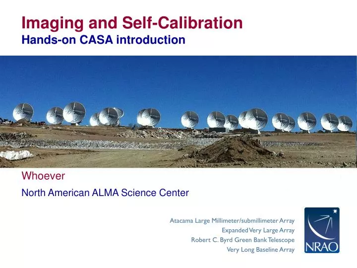
Imaging and Self-Calibration Hands-on CASA introduction. North American ALMA Science Center. Whoever. Imaging in CASA. CASA exposes i maging and deconvolution via the clean task Starting point: calibrated MS (“corrected” column, if present)

E N D
Imaging and Self-CalibrationHands-on CASA introduction • North American ALMA Science Center • Whoever
Imaging in CASA • CASA exposes imaging and deconvolutionvia the clean taskStarting point: calibrated MS (“corrected” column, if present) • Can be run interactively (using the viewer) or automaticallyInteractive allows on-the-fly clean boxing and stopping • Key decisions: • How to grid the data (image, cell size) • How to handle the frequency axis • What (if any) deconvolution to carry out • Selection and weighting of visibility data
clean • (Visibility) data selection • Treatment of spectral axis • Deconvolution (actual CLEANing) • Basic image (gridding) parameters • Weighting
clean: Imaging • image sizeTypically ~ primary beam area unless in special case • cell sizeSet this to place ~4-5 pixels across your PSF core • Weighting (“uniform”, “robust”, “natural”)Used to assemble visibilities into image, affect PSF/sensitivity • Optionally “taper” (smooth) the data to target resolution
clean: Imaging • Handling of spectral axis for cube:start, stop, width of plane • Define planes by channel • Define planes by velocity • Define planes by frequency • Handling of spectral axis for image: • “multifrequency synthesis” accounts for u-v position vs. frequency • (Optional) Deconvolution components can have spectral indexi.e., intensity dependent on frequency
clean: Deconvolution • Image reconstruction to account for imperfect u-v coverage • Basic Procedure: • Identify brightest spot in image • Subtract a point source with some fraction of that intensity • Add a corresponding point source to a “model” image • Proceed until no signal left in image • Convolve model with “clean beam” and add to residuals
Deconvolution Illustrated • Find brightest points in “dirty” image
Deconvolution Illustrated • Find brightest points in “dirty” image • Create model image containing a fraction of those flux points
Deconvolution Illustrated • Find brightest points in dirty image • Create model image containing a fraction of those flux points • Subtract model from data, leaving a residual
Find brightest points in dirty image • Create model image containing a fraction of those flux points • Subtract model from data, leaving a residual • Final product = residual + model • (convolved with restoring Gaussian beam)
model convolved w/ restorimg beam (log scale) residual (log scale) residual (linear scale) cleaned image (log scale)
model convolved w/ restoring beam (log scale) residual (log scale) residual (linear scale) cleaned image (log scale) restrict where the algorithm can search for clean components, with a mask
model convolved w/ restoring beam residual (log scale) 10 iterations residual (linear scale) cleaned image (log scale)
model convolved w/ restoring beam residual (log scale) 20 iterations residual (linear scale) cleaned image (log scale)
model convolved w/ restoring beam residual (log scale) 30 iterations residual (linear scale) cleaned image (log scale)
model convolved w/ restoring beam residual (log scale) 40 iterations residual (linear scale) cleaned image (log scale)
model convolved w/ restoring beam residual (log scale) 50 iterations residual (linear scale) cleaned image (log scale)
model convolved w/ restoring beam residual (log scale) 60 iterations residual (linear scale) cleaned image (log scale)
model convolved w/ restoring beam residual (log scale) 70 iterations residual (linear scale) cleaned image (log scale)
model convolved w/ restoring beam residual (log scale) 80 iterations residual (linear scale) cleaned image (log scale)
model convolved w/ restoring beam residual (log scale) 90 iterations residual (linear scale) cleaned image (log scale)
model convolved w/ restoring beam residual (log scale) 100 iterations residual (linear scale) cleaned image (log scale)
model convolved w/ restoring beam residual (log scale) 125 iterations residual (linear scale) cleaned image (log scale)
model convolved w/ restoring beam residual (log scale) 150 iterations residual (linear scale) cleaned image (log scale)
model convolved w/ restoring beam residual (log scale) 200 iterations residual (linear scale) cleaned image (log scale)
model convolved w/ restoring beam residual (log scale) 300 iterations residual (linear scale) cleaned image (log scale)
model convolved w/ restoring beam residual (log scale) 400 iterations residual (linear scale) cleaned image (log scale)
model convolved w/ restoring beam residual (log scale) 500 iterations residual (linear scale) cleaned image (log scale)
model convolved w/ restoring beam residual (log scale) 1000 iterations residual (linear scale) cleaned image (log scale)
model convolved w/ restoring beam residual (log scale) 1500 iterations residual (linear scale) cleaned image (log scale)
clean:Deconvolution cleaned image (log scale) dirty image (log scale)
clean: Deconvolution • Key decisions: • Constraining where the signal can be (clean boxing)Manually using the viewer or input as an image or region • Setting stopping thresholdTypically a small number times the RMS noise • Number of iterations allowedNot usually a good criteria to stop • Deconvolution algorithmBalance of Major/Minor cycles, etc.
Interactive clean • residual image in viewer • define a mask with R-click on shape type • define the same mask for all channels • or iterate through the channels with the tape deck and define separate masks
Interactive clean • perform N iterations • and return – every time the residual is displayed is a major cycle • continue until #cycles or threshold reached, or user stop
clean: Notes • clean restarts from existing fileswill first recompute residuals from model • The mask image, in particular, can be reusedBe careful of imsize – mask must match image • don’t hit ^C while imaging – this can do bad things to your MS
Self-Calibration in CASA • “Self-calibration” is just regular calibration • With a model of your source, you can calibrate on your source • Requires that your source is bright enoughNeeded to get sufficient S/N; get some S/N back time averaging. • Can be iterated as model improvesUsually phase-only selfcal first, amplitude selfcal later (if at all)
Self-Calibration in CASA Image your source, deconvolve build a model, place model in MSclean Measurement Set Initial Image Now has associated model. Calibrate to match data to modelgaincal Phase Calibration Table Amplitude Calibration Table Apply the new calibrationapplycal Measurement Set Improved corrected column. Re-image the better-calibrated data clean Improved Image
Self-Calibration in practice • Initial round of cleaningCareful not to overdo it: The self calibration can “lock in” artifacts • Experiment with solution interval (solint)S/N usually limiting concern, try pol. combination (gaintype=‘T’) • Inspect resulting solutionsLook for smooth trends of phase, amp. with time • May take multiple iterationsModel will successively improve, start with phase, then try amplitude
Your Turn • Follow the imaging CASA guide • http://casaguides.nrao.edu/index.php?title=TWHydraBand7_Im_SS12 • We have provided the full calibrated data setNo need to use this morning’s data, but you can if you like • Try: • Continuum imaging • Line imaging • Self-calibration and re-imaging • Moment map creation • Imaging your calibrators Ask if you need help!