Download
1 / 36
360 likes | 543 Views
PM Event Detection from Time Series. Contributed by the FASNET Community, Sep. 2004 Correspondence to R Husar , R Poirot Coordination Support by Inter-RPO WG Fast Aerosol Sensing Tools for Natural Event Tracking, FASTNET NSF Collaboration Support for Aerosol Event Analysis

E N D
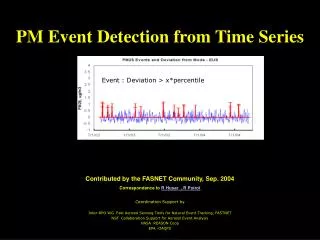
PM Event Detection from Time Series Contributed by the FASNET Community, Sep. 2004 Correspondence to R Husar , R Poirot Coordination Support by Inter-RPO WG Fast Aerosol Sensing Tools for Natural Event Tracking, FASTNET NSF Collaboration Support for Aerosol Event Analysis NASA REASON Coop EPA -OAQPS Event : Deviation > x*percentile
Temporal Analysis • The time series for typical monitoring data are ‘messy’; the signal variation occurs at various scales and the time pattern at each scale is different • Inherently, aerosol events are spikes in the time series of monitoring data but extracting the spikes from the noisy data is a challenging endeavor Typical time series of daily AIRNOW PM25 over the Northeastern US • The temporal signal can be meaningfully decomposed into a • Seasonal component with stable periodic pattern • Random variation with ‘white noise’ pattern • Spikes or events that are more random in frequency and magnitude • Each signal component is caused by different combination of the key processes: emission, transport, transformations and removal
Temporal Signal Decomposition and Event Detection EUS Daily Average 50%-ile, 30 day 50%-ile smoothing • First, the median and average is obtained over a region for each hour/day (thin blue line) • Next, the data are temporally smoothed by a 30 day moving window (spatial median - red line; spatial mean – heavy blue line). These determine the seasonal pattern. Event : Deviation > x*percentile Deviation from %-ile Average • Finally, the hourly/daily deviation from the the smooth median is used to determine the noise (blue) and event (red) components Mean Seasonal Conc. Median Median Seasonal Conc.
Seasonal PM25 by Region The 30-day smoothing average shows the seasonality by region The Feb/Mar PM25 peak is evident for the Northeast, Great Lakes and Great Plains This secondary peak is absent in the South and West
Northeast – Southeast Comparison • Northeast and Southeast differ in the pattern of seasonal and event variation • Northeast has two seasonal peaks and more events–values well above the median • Southeast peaks in September and has few values much above the noise Northeast Southeast
Causes of Temporal Variation by Region The temporal signal variation is decomposable into seasonal, meteorological noise and events Assuming statistical independence, the three components are additive: V2Total =V2Season +V2MetNoise +V2Event The signal components have been determined for each region to assess the differences Northeast exhibits the largest coeff. variation (56%); seasonal, noise and events each at 30% Southeast is the least variable region (35%), with virtually no contribution from events Southwest, Northwest, S. Cal. and Great Lakes/Plains show 40-50% coeff. variation mostly, due to seasonal and meteorological noise. Interestingly, the noise is about 30% in all regions, while the events vary much more, 5-30%
‘Composition’ of Eastern US Events • The bar-graph shows the various combinations of species-events that produce Reconstructed Fine Mass (RCFM) events • ‘Composition’ is defined in terms of co-occurrence of multi-species events (not by average mass composition) • The largest EUS RCFM events are simultaneously ‘events’ (spikes) in sulfate, organics and soil! • Some EUS RCFM events are events in single species, e.g. 7-Jul-97 (OC), 21-Jun-97 (Soil) Based on VIEWS data
Event Definition:Time Series Approach • Eastern US aggregate time series
Sulfate EUS Daily Average 50%-ile, 30 day 50%-ile smoothing Deviation from %-ile Event – Deviation > percentile value Mean Seasonal Conc. Median Seasonal Conc.
Temporal Pattern Regional Speciated Analysis - VIEWS • Aerosol species time series: • ammSO4f • OCf • ECf • SOILf • ammNO3f • RCFM Regions of Aggregation
Dust US Seasonal + spikes East – west events are independent East events occur several times a year, mostly in summer West events are lest frequent, mostly in spring East West
Dust Northeast asgasgasfg Southeast Southwest
Dust Northwest dfjdjdfjetyj Great Plaines S. California
Amm. Sulfate US wdthehreherh East West
Amm. Sulfate Northeast stheherheyju Southeast Southwest
Amm. Sulfate Northwest shheherh Great Plaines S. California
Organic Carbon US sdhdfhefheryj East West
Organic Carbon Northeast sdheherh Southeast Southwest
Organic Carbon Northwest erheryeyj Great Plaines S. California
Reconstructed Fine Mass US estrhertheryu East West
Reconstructed Fine Mass Northeast werty3rueru Southeast Southwest
Reconstructed Fine Mass Northwest wthwrthwerhtr Great Plaines S. California