Designing Experiments: What's Important and When to Get Help

1. Matthew Williams, Dept. of Statistics Designing Experiments:What's Important and When to Get Help

2. Learning Objectives • Develop an intuition for the basic concepts and vocabulary of Design of Experiments (DOE)‏ • Explain the idea behind Analysis of Variance (ANOVA), a method to analyze designed experiments. • Try some basic analysis with JMP, a common statistical software. • Recognize more sophisticated designs that may require advice or consultation.

3. Outline • Introduction • Purpose, Model, and Terminology • Steps in Planning, Conducting, and Analyzing an Experiment • Part 1 • Randomization, Replication, Local Control of Error (Blocking), and Confounding • Part 2 • ANOVA, Degrees of Freedom, Experimental Units and Observational Units, Sample Size and Power • Part 3 • Extensions and more advanced designs: multiple factors, nested factors, split plot designs, and random effects • Part 4 • Sequential Experimentation • How to learn more about DOE • Closing

4. Introduction to DOE • What is an experiment? • “A test or series of tests for which the process under study is under the active control of the experimenter” Stat5204 class notes • What is the purpose of a designed experiment? • exploration, confirmation, optimization • what else? • How does it differ from an observational study? • How do we establish cause and effect? • How do we assign treatments vs. how do we choose a representative sample? • What is our basic model? • Treatment Effects model • yij = μ + τi + εij • yij is the response, μ is overall average response, τi is the effect of the ith level of the factor of interest, εij is the random error or noise, and i = 1 to t treatments, and j = 1 to n observations.

5. Suppose we are interested in how road salt affects freshwater algae. We have 4 concentrations of salt and 20 samples of algae. Our response is growth. Our model is yij = μ + τi + εij yij is the response, algal growth, μ is the average growth for algae population, τi is the effect of salt concentration i on growth. εij is the random noise or error for each sample. i is the index for each concentration (1 to 4) and j is the index for each replicate (1 to 5) for each concentration. Example of the Model

6. Steps in Planning, Conducting, & Analyzing an Experiment (from Stat5204)‏ • Recognize and state the problem • Select the response variable • Choose the factors, levels, and ranges • Choose the design • Conduct the Experiment • Analyze the results (start by making some plots)‏ • Draw conclusions and make recommendations • LISA can help with any/all of these steps!

7. Part 1: Basic Design Principles • Randomization • Confounding • Local Control of Error: Blocking and ANCOVA • Replication • Generating some Designs in JMP

8. Randomization • Refers to the random assignment of treatments to samples (or experiments units)‏ and the random order in which trials are run • From a technical standpoint, it justifies the use of our tests and analyses. • Prevents assigning treatments in any systematic way, which could otherwise lead to bias (or accusations of bias). • Helps buffer against differences (unknown and unmeasured) between experimental units. Also known as “lurking” variables. • What else makes it useful?

9. Confounding • Confounding occurs when the individual effects of one or more factors cannot be separated from each other. • Example: Detergents and Washing Machines (Stat5204)‏ • 4 detergents and 4 washing machines • What would happen if each detergent was used only with one washing machine? • Could we determine the individual effects of either? • How could we make this design better?

10. Detergents A,B,C,D Machines 1,2,3,4 Confounding 1 2 3 4 Machines A B C D A B C D Replicates A B C D A B C D

11. Local Control of Error • Two Common Methods are: • Blocking: • Restrict randomization based on batches or blocks • Analysis of Covariance (ANCOVA): • Use a covariate that is measured for each EU, but not controlled (or randomly assigned)‏ • We Focus on Blocking because: • Basic blocking designs can be intuitive and require fewer assumptions • Analysis of designs with blocking is more straight-forward than with ANCOVA

12. Blocking • Start with an Example: We have a reagent that is only fresh for 6 hours and we have 24 samples, and 6 treatments. We can realistically process 6 samples for every batch of reagent. • Why shouldn't we use a completely randomized design? • Instead we use blocking: Assign each treatment once to each batch, repeat the whole thing 4 times

13. Blocking Batch 1 2 3 4 5 6 2 5 3 6 1 4 4 5 2 6 3 1 2 4 3 5 1 6 Treatments

14. Blocking • Look at the new model • yijk = μ + τi + βk + εijk • βk is the effect of the kth block on the response yijk • If blocks are not modeled, the block effect is absorbed into the modeled error and inflates it. • If replicate within each block you can also model any interaction between treatments and blocks

15. Part 1 JMP Example: Generating our two Designs • Complete Random Design (CRD)‏ • Model: yij = μ + τi + εij • Steps in JMP • DOE > Full Factorial Design • Under Response change name Y to Growth • Under Factors click on Continuous and Select 4-levels • Change name X1 to Salt • Click on Continue • Enter # of Replicates as 5. • Click on Make Table

16. Part 1 JMP Example: Generating our two Designs (cont.)‏ • Randomized Complete Block Design (RCBD)‏ • Model: yijk = μ + τi + βk + εijk • Steps in JMP • DOE > Custom Design • Under Response, change name Y to Yield • Under Factors, add a 6-level categorical • Rename X1 Treatment • Under Factors, add Blocking (Select other and type in 6 for runs per block)‏ • Rename X2 Batch • Continue • Change number of runs from 6 to 24 • Make Design, then Make Table

17. Part 2: Analysis of Designs • Intro to Analysis of Variance (ANOVA)‏ • How to Interpret Degrees of Freedom • Relating Degrees of Freedom, Sample Size, and Power • Experimental Units, Observational Units, and Sample Size • Exercises in JMP: Analyze RCBD, Power Calculations

18. Analysis of Variance (ANOVA)‏ • Idea: Partition the Total Variation (SSTot): • Between Treatments (SSTrt)‏ • Within Treatments (SSE)‏ • Compare standardized SSTrt and SSE • For our simple CRD model: • SSTot = SSTrt + SSE

19. ANOVA cont. • Test Statistic F0 Under H0 • If F0 is large enough, reject null • Check Assumptions of Normality and Constant Variance of Residuals

20. Degrees of Freedom • Degrees of Freedom: • Intuitively, number of samples (or EU's) that vary freely. Or the number of samples that can be used to estimate parameters (Need at least one EU per parameter). • Examples • SStotal has n-1 df (1 less because mean(y) is a restriction)‏ • SSTrt has t-1 df ( 1 less because sum of τ = 0)‏ • SSE has n-t df (t less since residuals add to zero for each of the t groups)‏

21. Degrees of Freedom, Sample Size, and Power • Power: • The ability to reject the null hypothesis (treatment effects 0) when the alternative hypothesis is true. • When Ho is wrong, how often you reject Ho depends on the power of your design • Sample Size and df • Concept: When increase Sample Size, the df that can be used to estimate the Error increase. This means the variance estimate of our model (MSE = SSE/df) generally gets smaller. So our chances of detecting a true difference get better • Technically, Power and Sample Size calculations depend true values of τ(unknown) variance of the error (unknown)‏ • Except for the most basic case, we can't do this calculation without software.

22. Experimental Units vs. Observational Units • Experimental Unit (EU)‏ • The unit to which a treatment combination is applied • Sample size and df come from EU! • Observational Unit (OU)‏ • The unit that is measured by the researcher. • If more OU than EU, can estimate observational or measurement errors • Sometimes they are the same, and sometimes they are not! • For every design, identify which is which!

23. EU vs OU Illustration • Fish Tank Example: We have 6 tanks each with 5 fish. We have 3 treatments, each applied to 2 tanks. We measure the growth of each fish in every tank. What are the EU's and what are the OU's? • What's the problem if we assume OU = EU? (What are we assuming?)‏ Trt 1 Trt 2 Trt 3

24. Part 2 JMP Examples • Simple RCBD example • Herbicide and yield of plants (weight)‏ • Data from http://www.stat.sfu.ca/~cschwarz/Stat-650/Notes/MyPrograms/ • Steps in JMP • First create the design • Input the data • In the Table right click Model > Run Script • Click Run Model • Simple Power Calculation (red triangle options)‏

25. Part 2 JMP Examples • Simple Power Calculation • DOE > Sample Size and Power • Select Two-sample Means • Fill in Values, leaving either Sample Size of Power Blank • If both Blank, JMP makes a plot for you.

26. Part 3: More Complicated Designs • Multiple factor designs • Incomplete Block Designs • Nested and Split Plot Designs • Fixed vs. Random Effects • Examples in JMP: Split Plot Example

27. Multiple Factor Designs • 2 Factor Case • Additive Model (Assumes no interaction between levels of different treatments)‏ • Non-additive (Interaction) Model • Analysis with 2-Way ANOVA • Now have SSA, SSB, SSAB, and SSE • F-statistic is simply MS(Factor)/MSError • Adding blocking or more Factors is also straight-forward • Accessibility: • Take an ANOVA course and/or have a good reference and you should be fine (But still feel free to ask for help!)‏

28. Multiple Factor Example • 2 Factor Case • 4 Catalysts (A,B,C,D) and 3 Temperatures (450, 475, 500)‏ • Each Catalyst and Temperature combination should appear at least once for the Additive model and twice for the Interaction model • In general, a balanced design (same number of replications for each combination) has the best properties

29. Incomplete Block Designs • When the number of treatments > number of EU in each block • You can’t run every treatment in each block • Balanced Design • All treatments occur the same number of times and pairs of treatments (in each block) occur the same number of times • Variance of estimates is about the same for each treatment • Incomplete Design • Some treatments occur more times than others and some pairs of treatments occur more times than others • Some estimates will have less variance than others. • Accessibility: • Calculation and interpretation of estimates is more difficult. • Recommend a good reference and consulting an expert/experienced practitioner

30. Balanced Incomplete Block Design Example • BIBD • We have 4 treatments, but can only run 3 per day. Conditions change day to day, due to variations in raw materials. Thus we decide to block by day. We can't fit in each treatment every day so we use a BIBD. Days 1 2 3 1 2 4 1 3 4 2 3 4 Treatments

31. Nested Designs (2 or More Factors)‏ • Nested Designs vs. Crossed Designs • Crossed: Every combination of factor levels is present • Nested: Some levels of one factor are only present within certain levels of another factor • Example: • We are interested in testing the effects of operators and manufacturing locations on yield. • Should this be a nested or crossed design? (Hint: Can we use the same operators for every location?)‏ • We'd say operator is “nested within” manufacturing location • Accessibility: • If you are proficient in ANOVA and have a good reference, give it a try! • Nested Designs can exist in combination with other designs: Blocking, Factorial, etc. For complex designs, get help

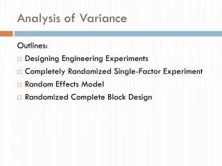
32. Split Plot Designs (2 or More Factors)‏ • Split-Plot Designs • EU’s are different for different factors (hard to change and easy to change)‏ • EU’s for one factor are OU’s for another! • Visual Example: Effects of Temperature (A,B,C) and carbon content (1,2,3,4) for steal plates. Carbon content easy to change, Temperature for tempering is hard to change. 1 2 3 4 3 4 2 1 3 1 4 2 2 3 1 4 4 2 3 1 3 2 4 1 A C A B B C

33. Split Plot Designs (2 or More Factors)‏ • Accessibility: • Similar to Nested Designs • Simple case: Good ANOVA skills and a good reference, give it a try! • Complex Designs: get help.

34. Random vs. Fixed Effects • Fixed Effect (What we've seen so far)‏ • The levels of the treatment are the only ones we care about. We can only make inference about the levels we set • Example: We have three settings on our temperature controls and we only want to learn about the effects of these three settings • Random Effect • The levels of the treatments are selected randomly from a larger population. We are not interested in any properties of the levels we observe, but instead are interested in the population of possible levels. • Example: We have 100 operators in our plant. We randomly select 5 as our levels and want to learn about the effects of the the whole population of 100. • Accessibility: • Simple Random Effects model are simple to analyze, however models with mixtures of Random and Fixed Effects or many Random Effects can become complicated. Recommend a course in ANOVA and a good reference

35. Part 3 JMP Examples • Simple RCBD example • Method and Temperature on Paper Strength • Data from http://www.stat.sfu.ca/~cschwarz/Stat-650/Notes/MyPrograms/ • Steps in JMP • First create the design • DOE > Custom Design • Add two factors (Method and Temperature)‏ • Make Method factor Hard • Continue, Make Design, Make Table • Input the data • In the Table right click Model > Run Script • Click Run Model

36. Part 4: Final Thoughts • Sequential Experimentation • How to Learn more about DOE

37. Sequential Experimentation • Used in Industry all the time • Avoid using more than 25% of budget on one experiment • Design experiments to test methodology and experimental setup, before running the main experiment of interest. • Initial estimates of MSE can help with power/sample size estimates • Also use as a screening device if have too many factors

38. How to Learn More about DOE • Stat5204 : Experimental Design and Analysis • Lots of Textbooks out there: • I used Montgomery (Design and Analysis of Experiments, ISBN-13: 978-0471487357)‏ • Other common ones? • Several Statistics Faculty are work in Design • LISA is here to help you (of course!)‏

39. Closing • Learning Objectives? • Other Questions? • Break for refreshments and small group discussion with consultants

40. Learning Objectives • Develop an intuition for the basic concepts and vocabulary of Design of Experiments (DOE)‏ • Explain the idea behind Analysis of Variance (ANOVA), a method to analyze designed experiments. • Try some basic analysis with JMP, a common statistical software. • Recognize more sophisticated designs that may require advice or consultation.