Download

1 / 35
350 likes | 529 Views
Response Surface Method Principle Component Analysis. Daniel Baur ETH Zurich, Institut für Chemie- und Bioingenieurwissenschaften ETH Hönggerberg / HCI F128 – Zürich E-Mail: daniel.baur@chem.ethz.ch http://www.morbidelli-group.ethz.ch/education/index . Definitions.

E N D
Response Surface MethodPrinciple Component Analysis Daniel BaurETH Zurich, Institut für Chemie- und BioingenieurwissenschaftenETH Hönggerberg / HCI F128 – ZürichE-Mail: daniel.baur@chem.ethz.chhttp://www.morbidelli-group.ethz.ch/education/index Daniel Baur / Numerical Methods for Chemical Engineers / RSM & PCA
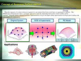
Definitions • The response surface method is a tool to • Investigate the repsonse of a variable to changes in a set of design or explanatory variables • Fine the optimal conditions for the response • Example: Consider a chemical process where the yield is a (unknown) function of temperature and pressure, and you want to maximize the yield Daniel Baur / Numerical Methods for Chemical Engineers / RSM & PCA
COVT Approach • COVT stands for «Change One Variable per Time» • This approach makes a fundamental assupmtion: • Often, experimentation starts in a region far from the optimum • Example: We do not know the response surface for Y(T,P), but we start investigating it by first changing T, then P. Changing one parameter at a time is independent of the effects of changes in the others. This is usually not true! Daniel Baur / Numerical Methods for Chemical Engineers / RSM & PCA
Optimum ??? Optimum !!! COVT Approach (Example) T 50 Contour curves for the yield (Y) 60 70 Design of experiments 80 Starting point P Daniel Baur / Numerical Methods for Chemical Engineers / RSM & PCA
Optimum 2k Factorial Design T 50 Contour curves for the yield (Y) 60 Design of experiments 70 80 +1 Initial investigation starts with a first order approximation of the response surface -1 +1 -1 P Daniel Baur / Numerical Methods for Chemical Engineers / RSM & PCA
Example: Plastic Wrap • The strength of a plastic wrap (Y) is a function of the sealing temperature (T) and the percentage of polyethylene additive (P). A process engineer tries to make the wrap as strong as possible (maximize Y). • The response function (unknown to the engineer!) reads: • Starting conditions: • T = 140 C, P = 4.0% • Optimal conditions (analytical): • T = 216 C, P = 9.2% Daniel Baur / Numerical Methods for Chemical Engineers / RSM & PCA
Optimum Starting point Ture Response Surface Daniel Baur / Numerical Methods for Chemical Engineers / RSM & PCA
+1 -1 +1 -1 2k Factorial Design Initial regression model: Daniel Baur / Numerical Methods for Chemical Engineers / RSM & PCA
22 Factorial Design True Response Surface Contour Curves of Y Daniel Baur / Numerical Methods for Chemical Engineers / RSM & PCA
First Order Regression Regressed Response Daniel Baur / Numerical Methods for Chemical Engineers / RSM & PCA
+1 -1 +1 -1 Central point does not influence the regression of the slope 2k Factorial Design with Center Point Initial regression model: Daniel Baur / Numerical Methods for Chemical Engineers / RSM & PCA
22 Factorial Design with Center Point True Response Surface Contour Curves of Y Experimental Responses Daniel Baur / Numerical Methods for Chemical Engineers / RSM & PCA
First Order Regression Regressed Response Daniel Baur / Numerical Methods for Chemical Engineers / RSM & PCA
Curvature • The center point can give us an indication about the curvature of the surface and its statistical significance • If there is no curvature and the linear model is appropriate in the region of interest, then the average value of the experimental responses in the center point(s) and in all the corners is roughly equal (within the standard deviation) C- C+ Daniel Baur / Numerical Methods for Chemical Engineers / RSM & PCA
Tukey-Anscombe Plot Daniel Baur / Numerical Methods for Chemical Engineers / RSM & PCA
Steepest Ascent Direction Experimental Points Contour Lines of the Regressed 1st order Surface Steepest Ascent Direction t p Daniel Baur / Numerical Methods for Chemical Engineers / RSM & PCA
Steepest Ascent Direction Daniel Baur / Numerical Methods for Chemical Engineers / RSM & PCA
Monodimensional Search Monodimensional search Steepest Ascent Direction Daniel Baur / Numerical Methods for Chemical Engineers / RSM & PCA
Monodimensional Search Experimental points True Response along the steepest ascent direction Daniel Baur / Numerical Methods for Chemical Engineers / RSM & PCA
New 2k Factorial Design 22 Factorial Design with Center Points Maximum of response surface (unknown) Maximum from the monodimensional search Daniel Baur / Numerical Methods for Chemical Engineers / RSM & PCA
22 Factorial Design with Center Points True response surface Experimental Points Daniel Baur / Numerical Methods for Chemical Engineers / RSM & PCA
First Order Regression Regressed Response Daniel Baur / Numerical Methods for Chemical Engineers / RSM & PCA
Central Composite Design r = 21/2 Central Composite Design 2k Factorial Design At least three different levels are needed to estimate a second order function Daniel Baur / Numerical Methods for Chemical Engineers / RSM & PCA
Central Composite Design Daniel Baur / Numerical Methods for Chemical Engineers / RSM & PCA
Central Composite Design Tukey-AnscombePlot Daniel Baur / Numerical Methods for Chemical Engineers / RSM & PCA
Response Surface Method Algorithm • Use 2k factorial design to generate linearization points around a starting point x(0), where k is the number of variables • Fit a linear regression model • Check if the curvature is large. If so, jump to point 7. • If you think you are far from the maximum, you can try smaller steps. • Find the steepest ascent direction Daniel Baur / Numerical Methods for Chemical Engineers / RSM & PCA
Response Surface Method Algorithm (Continued) • Conduct experiments at points along the steepest ascent direction • When a maximum in the response variable occurs, setx(0) = x(k) and go back to point 1. • Perform a central composite design around the current point. Fit a second order linear regression. • Find the extremum of the regression curve by setting the Jacobian equal to zero and solving the resulting linear system • Check that J is negative definite (all eigenvalues < 0) to ensure a maximum in the function Daniel Baur / Numerical Methods for Chemical Engineers / RSM & PCA
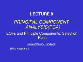
p k X A n n Principal Component Analysis (PCA) • Consider a large sets of data (e.g., many spectra (n) of a chemical reaction as a function of the wavelength (p)) • Objective: Data reduction: find a smaller set of (k) derived (composite) variables that retain as much information as possible Daniel Baur / Numerical Methods for Chemical Engineers / RSM & PCA
PCA • PCA takes a data matrix of n objects by p variables, which may be correlated, and summarizes it by uncorrelated axes (principal components or principal axes) that are linear combinations of the original p variables • New axes = new coordinate system • Construct the Covariance Matrix of the data (which need to be centered), and find its eigenvalues and eigenvectors Daniel Baur / Numerical Methods for Chemical Engineers / RSM & PCA
PCA in Matlab • There are two possibilities to perform PCA with Matlab: • 1) Use Singular Value Decomposition: • [U,S,V]=svd(data); • where U contains the scores, V the eigenvectors of the covariance matrix, or loading vectors. SVD does not require the statistics toolbox. • 2) [COEFF,Scores]=princomp(data);is a specialized command to perform principal value decomposition. It requires the statistics toolbox. Daniel Baur / Numerical Methods for Chemical Engineers / RSM & PCA
Exercise 1 • A chemical engineer tries to optimize the a reaction by maximizing the yield. There are two variables which influence the yield: The reaction time and the reaction temperature. Currently, the reaction is carried out for 35 minutes at 155 F, resulting in a yield of about 40%. • Three sets of experiments were conducted, given in the data files reactionYield-1 through 3. The datasets are structured identically, with the first two columns being time and temperature, the third and fourth column the same variables in coded units (-1, +1, etc.) and the last column is the yield y. Daniel Baur / Numerical Methods for Chemical Engineers / RSM & PCA
Assignment 1 • The first data set is near the current operating point. • Fit a first order (planar) surface to the data. • What is the direction of the steepest ascent? • Plot the operating conditions, experimental design points and the direction you found in the parameters plane Time vs. Temperature. • The second data set contains more experiments in the direction found in part 1. • Plot the data (for example as Yield vs. Temperature) and find out where the yield reaches a maximum along this direction. Daniel Baur / Numerical Methods for Chemical Engineers / RSM & PCA
Assignment 1 (Continued) • The maximum in 2. is used for another first order design, this data is found in the third data set. • Show that the curvature of the response surface is significantly different from zero. • The data from 3. is now extended to a central composite design. Fit a second order (quadratic) response surface to the data and calculate the maximum analytically. • If you are using LinearModel, you can specify second order terms in the modelspec by using the * and ^ operators, for example'y ~ a*b' will incorporate a, b and a*b, and 'y ~ a^2' will use the quadratic term. So for two variables a and b, the modelspec string for a second order linear regression will read'y ~ a^2 + a*b + b^2' Daniel Baur / Numerical Methods for Chemical Engineers / RSM & PCA
Assignment 2 • The dataset d_react contains data of IR spectra measured during a chemical reaction (122 x 700). The first row contains the wavelength, all other rows the spectra. • Create a matrix centeredData, obtained by centering the data, i.e. subtracting the column mean from each column. What can observe when looking at the centered spectra? What distinguishes the different observations (spectra) regarding the different variables (wavelengths)? • Perform singular value decomposition on the centered data. The U matrix of this decomposition contains the «scores» in terms of PCA. • Use [U,S,V] = svd(centeredData); Daniel Baur / Numerical Methods for Chemical Engineers / RSM & PCA
Assignment 2 (Continued) • Plot the first 3 scores in a scatterplot matrix using the plotmatrix function. • Plot the first three loading vectors (columns of V) versus the wavelength. What can you observe? Compare with what you have seen in point 2. Daniel Baur / Numerical Methods for Chemical Engineers / RSM & PCA