Production Process & Cost Baye Chapter 5

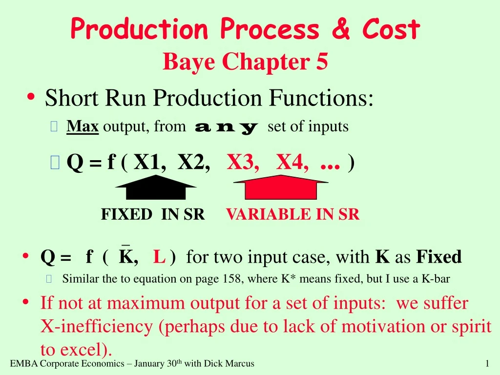
1. Production Process & CostBaye Chapter 5 • Q = f ( K, L ) for two input case, with K as Fixed • Similar the to equation on page 158, where K* means fixed, but I use a K-bar • If not at maximum output for a set of inputs: we suffer X-inefficiency (perhaps due to lack of motivation or spirit to excel). • Short Run Production Functions: • Max output, from a n y set of inputs • Q = f ( X1, X2, X3, X4, ... ) FIXED IN SR VARIABLE IN SR _

2. Average Product = Q / L (p. 159) • output per labor • Marginal Product =Q / L (p. 159) • output attributable to last unit of labor applied • Similar to profit functions, the Peak of MP occurs before the Peak of average product • When MP = AP, we’re at the peak of the AP curve

3. Short Run Production FunctionSee also figure 5.1 on page 160 Marginal Product Average Product

4. When MP > AP, then AP is RISING • IF YOUR MARGINAL GRADE IN THIS EMBA CLASS IS HIGHER THAN YOUR AVERAGE GRADE POINT AVERAGE SO FAR, THEN YOUR G.P.A. IS RISING • When MP < AP, then AP is FALLING • IF YOU JOINED THE PITTSBURGH STEELER’S FOOTBALL TEAM, YOUR MARGINAL WEIGHT IS LESS THAN AVERAGE WEIGHT, SO THE TEAM’S AVERAGE WEIGHT WOULD DECLINE. • When MP = AP, then AP is at its MAX • IF THE NEW HIRE IS JUST AS EFFICIENT AS THE AVERAGE EMPLOYEE, THEN AVERAGE PRODUCTIVITY DOESN’T CHANGE

5. Law of Diminishing Returns INCREASES IN ONE FACTOR OF PRODUCTION, HOLDING ONE OR OTHER FACTORS FIXED, AFTER SOME POINT, MARGINAL PRODUCT DIMINISHES. Total Output A SHORT RUN LAW point of diminishing returns input

6. Fill in the following table Number of units Total Output MP AP 3 ---- unknown 30 4 ---- 20 --- 5 130 ----- --- 6 ---- 5 --- 7 ---- ---- 19.5

7. Long Run Production Functions • All inputs are variable greatest output from any set of inputs • Q = f( K, L ) is two input example. • MP of capital and MP of labor are the derivatives of the production function MPL = Q /L • MP of both inputs decline as more input is applied, other things equal

8. Cobb-Douglas Production Functions: Q = A • K  • L page 166-7 This is a Cobb-Douglas Production Function IMPLIES: Can be IRS, DRS or CRS: if  +  1, then CRS if  + < 1, then DRS if  + > 1, then IRS Coefficients are elasticities  is the capital elasticity of output  is the labor elasticity of output, which are EK and E L

9. Problem with a given LR Production Function • Suppose: Q = 1.4 L .70 K .35 Is the production function CRS? What is the labor elasticity of output? What is the capital elasticity of output? What happens to Q, if L increases 3% and capital is cut 10%? Q* = EL• L* + EK • K* = .7(+3%) + .35(-10%) = 2.1% -3.5% = -1.4%

10. Isoquants (pp. 169-177) • Isoquants: Equal Quantities • locus of all input combinations of the same quantity of output. • Can use mostly capital • Can use mostly labor • Can use some of both K 1 Isoquant 2 3 L

11. In the LONG RUN, ALL factors are variable Q = f ( K, L ) ISOQUANTS -- locus of input combinations which produces the same output SLOPE of ISOQUANT is ratio of Marginal Products ISOQUANT MAP Isoquants & LR Production Functions K Q3 B C Q2 A Q1 L

12. The Objective is to Minimize Cost for a given Output ISOCOST lines are the combination of inputs for a given cost MRTS is MPL/MPK See page 169 for the equimarginal principle. Equimarginal Principle Produce where MPL / W = MPK / R where marginal products per dollar are equal Optimal Input Combinations in the Long Run at E, slope of isocost = slope of isoquant E K Q1 L

13. Is the following firm EFFICIENT? Suppose that: MP L = 30 MP K = 50 W = 10 R = 25 Labor: 30/10 = 3 Capital: 50/25 = 2 A dollar spent on labor produces 3, and a dollar spent on capital produces 2. SO:USE RELATIVELY MORE LABOR If spend $1 less in capital, output falls 2 units, but rises 3 units when $1 is spent on labor ! Use of the Efficiency Criterion

14. Economies of Scale • CONSTANT RETURNS TO SCALE (CRS) • doubling of all inputs doubles output • INCREASING RETURNS TO SCALE (IRS) • doubling of all inputs MORE than doubles output • DECREASING RETURNS TO SCALE (DRS) • doubling of all inputs DOESN’T QUITE double output

15. Reasons for IRS 1.SPECIALIZATION • Adam Smith’s pin factory 2. INVENTORY ECONOMIES 3. SIZE-VOLUME LAWS • volume rises by cube 4. AVOID INHERENT INDIVISIBILITIES 5. QUANTITY DISCOUNTS • pecuniary and non-pecuniary quantity discounts

16. Reasons for DRS 1. INFLEXIBILITY e.g., Military or Post Office 2. HIGH COSTS OF MANAGING LARGE GROUPS use of divisions at G.M. 3. CAPACITY TO MAKE BIG DECISIONS IS LIMITED Austrian Argument--there is diminishing returns to the C.E.O. which cannot be completely delegated

17. Economies of Scope • FOR MULTI-PRODUCT FIRMS, COMPLEMENTARY IN PRODUCTION MAY CREATE SYNERGIES • especially common in Vertical Integration of firms • TC( Q 1 + Q 2) < TC (Q 1 ) + TC (Q 2 ) = Cost Efficiencies +

18. Estimating Production Functions Choice of data sets • cross section best for long run analysis • output and input measures from a group of firms • output and input measures from a group of plants • time series best for short run analysis • output and input data for a firm over time

19. Choice of Functional Form • Linear ? Q = a • K + b • L • is CRS (see page 165) • marginal product of labor is constant, MPL = b • can produce with zero labor or zero capital • isoquants are straight lines -- perfect substitutes in production K Q3 See Figure 5-4 panel A Q2 Q1 L

20. Leontief Production Functions K • Q = F(K,L) = min{bK, cL} • This is also known as fixed proportions • Must have one typists and one computerized word processing machine to produce written work. Q3 Q2 Q1 L Figure 5.4, panel B

21. Multiplicative -- Cobb Douglas Production Function Q = A • K  • L  • IMPLIES • Can be CRS, IRS, or DRS • MPL = • QL • MPK =  • Q • Cannot produce with zero L or zero K • Log linear -- double log Ln Q = a + • Ln  • Ln L • coefficients are elasticities

22. ANSWERS Problem Suppose the following production function is estimated to be: ln Q = 2.33 + .19 ln K + .87 ln L • Take the sum of the coefficients • .19 + .87 = 1.06 • which shows that this production function is IRS. • 2. Use the Percentage Rate of • Change Rules (Page 3 in notebook, see slide 12). • Q* = E K • K* + E L • L* • Q* = (.19)•(-5%) + (.87)•(+2%) • = +.79 R 2 = .97 Q U E S T I O N S: 1. Is this CRS? 2. If L increases 2% & K decreases 5%, what happens to output?

23. Figure 5-9: A Wage Increase K • If wages rise, the iscost line shifts inward from A to C • Pure substitution, from A to B B A C L L2 L1 Optimal amount of labor shrinks.

24. Cost – beginning page 177 An Assortment of Cost Concepts 1. Opportunity Cost -- value of next best alternative use. 2. Explicit vs. Implicit Cost -- actual prices paid vs. opportunity cost of owner supplied resources. 3. Accounting Profits vs Economic Profits: Economic Profits = Accounting Profits - Normal Profits

25. 4. Sunk Costs-- already paid for, or there is already a contractual obligation to pay 5. Incremental Cost - - extra cost of implementing a decision =  TC of a decision 6. Marginal Cost-- cost of last unit produced =  TC/Q 7. Time -- an important dimension of costs in the short run (SR) and long run (LR).

26. Two primary components of cost: a. input prices -- amount spent to purchase inputs b. productivity -- how productive are those inputs SHORT RUN COST FUNCTIONS 1. TC = FC + VC fixed & variable costs 2. ATC = AFC + AVC = FC/Q + VC/Q

27. Short Run Cost GraphsFigure 5.12, page 182 MC ATC 3. 1. AVC AFC AFC Q Q MCintersects lowest point of AVC and lowest point of ATC. When MC < AVC, AVC declines When MC > AVC, AVC rises 2. AVC Q

28. Typically use TIME SERIES data of cost Quadratic Total Cost (to the power of two) TC = C0 + C1 Q + C2 Q2 Write the TC equation Find AC function Find MC function REGR c1 1 c2 c3 EstimatingShort Run Cost Functions Minitab Output: Predictor Coeff StdErr T-value Constant 1000 300 3.3 Q -50 20-2.5 Q-squared 10 2.5 4.0 R-square = .91 Adj R-square = .90 N = 35

29. Long Run Cost Functions: Envelope of SRAC curvesFigure 5.13, page 186 Ave Cost SRAC-small capital SRAC-med. capital SRAC-big capital LRAC--Envelope of SRAC curves Q

30. Long Run Costs SRMC1 • In Long Run, ALL inputs are variable • LRAC • long run average cost • ENVELOPE of SRAC curves • LRMC is FLATTER than SRMC curves LRMC SRAC1 LRAC Q

31. The Survivor Techniqueto study LR cost curves • The Survivor Technique examines if some firm sizes are tending to succeed over time and if other sizes are declining. • This is a sort of Darwinian survival test for firm size. • Presently many banks are merging, leading one to conclude that small size offers disadvantages at this time. • Dry cleaners are not particularly growing in average size, however. George Stigler, Nobel laureate 1911-1991

32. The Organization of the Firm Baye Chapter 6 The Rôle of the Firm Business classes presume production occurs in a firm • Yet we can & do produce things at home • Suppose that all goods were produced in households • We’d be limited by size of household • Suppose there exist some economies of scale in organizational size • Let two households merge • if more productive, then other households will emulate them • Four households merge • if true for 2 households, why not true if 2 million households merged? • problems arise as the size of the collective grows • Less Personal Incentives • Who is in Charge? • Disagreements & Conflict Resolution Issues

33. How is garbage priced? What would you expect to find? What if food were delivered by cities to people in the same way? What do you think of a fee per bag of garbage? What will happen to the weight of garbage? Do deposits on bottles and cans affect behavior? How could we encourage more recycling? What does your community do? Discussion of especially Question #4 on page 170. The Trashman ComethMBN Chapter 26

34. Entrepreneurship • Synonym is CONTRACTOR • contractor monitors production • hires labor at fixed rates • purchases materials • receives the residual • This is a firm - contractor - entrepreneur • 87% of all production by corporations • remaining 13% in proprietorships & other

35. Competing Views onFirm Behavior & Conflicts Over Ownership 1. Standard View a. Firms are owned by shareholders, hence transfers of ownership are easy, and potentially perpetual. b. Firms provide limited liability up to amount invested. Note that as firm's merge, they dilute the effectiveness of the limited liability. (Partnerships & Proprietorships don't have this protection). c. Firms allow separation of management and ownership.

36. d. The objective for firm managers is to maximize the present value of the stream of profits: PV =  [ Profitst /(1+rt)t ] The standard view is less help dealing with conflicts of interest within firms. 2. Principal-Agent Theoryconflicts arise due to different objectives of agents and principals. • The agents (managers) may wish to maximize leisure and minimize risk, • whereas the principal (shareholders) may wish hard work and high risk-return investments.

37. Free Rider Problem • Example:an employee knows that working hard helps the whole firm, and helps himself only a little. Why not let the other workers be grinds and take it easy (be a free rider)? • Principal-Agent problems may lead to: •Risk Avoidance in Managers • Managers have Short Time Horizons • Sales Maximization • High Levels of Social Amenities at the Work Site • Satisficing or Sufficing Behavior • COMMENT: Competition among managers and competition among firms in acquisition tend to limit non-profit maximizing behavior.

38. Attempt is to align manager's interests with shareholders by: profit incentives, ownership positions, or options. • Creation of profit centers and transfer prices to create rewards and incentives. • But ownership of a little stock does not eliminate the free rider problem, that a lost $1 of profit "hurts" a partial owner only a tiny bit. • The principle-agent approach can also explain why some firms are vertically integrated and others contract-out many steps in production.

39. example: Vertical Integration(G.M. Corporation) GM Car production division transfer prices Fisher Body • Who wants a low transfer price? • Who wants a high transfer price? • Internal Conflict

40. 3. Transaction Cost Economics • Ronald Coase- use of the price system is costly • Nobel Prize winner in economics • Use of internal price systems (transfer pricing) are also costly. • When do we integrate activities? • When the costs are lower than contracting through separate firms. • When do we spin off tasks? • When the costs are low for explicit contracts • Few steps involved • Easy to observe quality of workmanship

41. 4. Nexus of Contracts Management Shareholders Employees Bondholders Customers Government Suppliers All parties have “interests” in the firm FIRM

42. The "owners" of a firm are broadly defined as those who have relationships with the firm via contracts. • This includes bondholders, management, and employees. • The residual claimant (shareholders) have only a liquidation lien on what is left over. • Most managers and employees think of themselves and "their" firm. • COMMENT: All four views of corporate life are correct in different settings.