Download
1 / 15
160 likes | 283 Views
AAMW. AAIW. NADW. CDW. AABW. Overturning Streamfunction. AAMW. AAIW. NADW. CDW. AABW. Overturning Streamfunction with Parameterized Eddies. Overturning Response to 20% Increase in Winds after 20 years. Explicit Eddies. Parameterized Eddies.

E N D
AAMW AAIW NADW CDW AABW Overturning Streamfunction
AAMW AAIW NADW CDW AABW Overturning Streamfunction with Parameterized Eddies
Overturning Response to 20% Increase in Winds after 20 years Explicit Eddies Parameterized Eddies
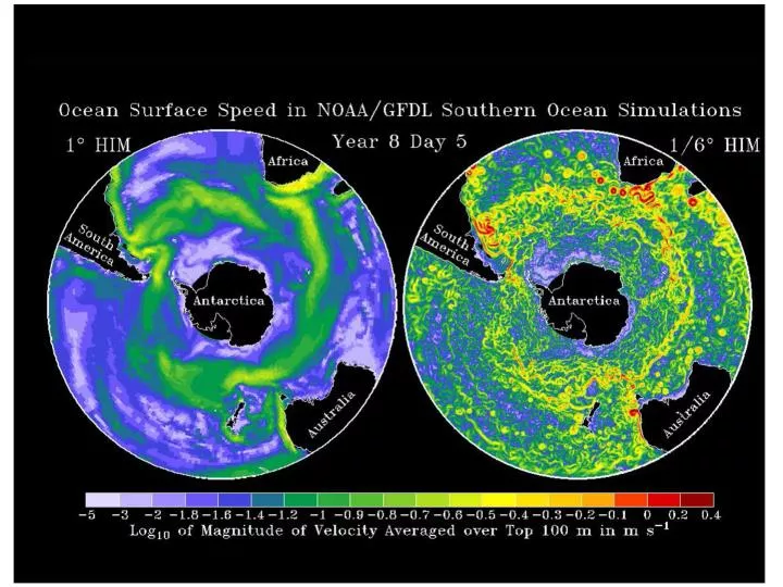
Summary of MESO Findings The Southern Ocean eddy dynamics are of leading order importance in regulating the watermasses that fill the deep ocean. The fine and coarse resolution models are qualitatively similar in many regards, but the models differ in two key ways: • The explicit eddies contribute a poleward extension of the subtropical overturning cell and heat fluxes that may be difficult to parameterize diffusively. • The overturning response to wind forcing changes is substantially weaker and has a shallower compensating flow than with parameterized eddies. “Eddy-saturation” theories seem appropriate. Eddy-permitting ocean models should be used to evaluate key climate predictions. Ref: Hallberg & Gnanadesikan, JPO 2006.
Numerical Diapycnal Diffusion in Ocean Models • Non-rotated horizontal diffusion operator leads to “Veronis effect”, • The same issue arises with a nonrotated biharmonic diffusion (Roberts & Marshall 1998) • Avoided in Z-coordinate models by using Gent/McWilliams closure (Gent et al. 1995) and rotating the diffusion tensor to align with isopycnals (Griffies et al. 1998) • Advective truncation errorslead to spurious watermass modification in Z-coordinate and s-coordinate models (Griffies et al. 2000). • In coarse resolution models, diffusion can be acceptably small, provided that western boundary currents are well resolved. • The cascade of variance to small scales in eddy rich models leads to diffusivities of order 1 cm2 s-1. • Avoiding advective spurious mixing in Z- and s- coordinate models is an area of active research, but there is no known solution without suppressing eddy variability. • Isopycnal coordinate models avoid numerical diapycnal diffusion at all resolutions (apart from effects of the nonlinear equation of state).
Numerical Diapycnal Diffusion in Low Resolution Gyresfrom Griffies, Pacanowski, and Hallberg, Mon. Wea. Rev., 2000 Physical Diffusion 10-5 m2 s-1 Veronis Effect Marginally Resolved Western Boundary Currents Well Resolved Western Boundary Currents Diagnosed effective diffusivity from advective truncation errors.
Numerical Diapycnal Diffusion in Eddy-Rich Z-modelsfrom Griffies, Pacanowski, and Hallberg, Mon. Wea. Rev., 2000 • In a representative channel flow, diagnosed numerical diapycnal diffusion is unacceptably large. • Eliminating this diffusion requires: (A) unexploited higher resolution (B) suppressing the cascade of variance, or (C ) much better approaches to tracer advection? • Lee, Coward, & Nurser (JPO 2002) find similarly large numerical diapycnal diffusion in an analysis of a ¼o global ocean-only model. • Marchesiello et al. (Ocean Modelling 2009) report that the problem is even worse in s-coordinate models, peaking when the eddies start to be well resolved, only becoming “acceptable at resolutions finer than 1 km”. Diffusivity from Quicker at 1/6° Res. 0 Diagnosed spurious diffusion 200 400 Depth (m) 600 800 1000 Kd=10-5 m2 s-1 1200 Diagnosed Diapycnal Diffusivity (cm2 s-1)
1/8° Global Isopycnal-Coordinate Model Based on CM2G May 1, Year 5
Discussion? • Do we need to explicitly resolve eddies in ocean climate models? • Is spurious diapycnal mixing a serious problem in long-term simulations with eddy-rich ocean climate models? • Are there good solutions to avoiding spurious diapycnal mixing (apart from using isopycnal coordinates)?