Download
1 / 33
330 likes | 432 Views
Bluing of Aerosols near Clouds: Results from a Simple Model and MODIS Observations. Alexander Marshak (GSFC) Tam á s V á rnai and Guoyong Wen (UMBC/GSFC) Lorraine Remer and Bob Cahalan (GSFC) Jim Coakley (OSU) and Norman Loeb (LRC). What happens to aerosol in the vicinity of clouds?.

E N D
Bluing of Aerosols near Clouds: Results from a Simple Model and MODIS Observations Alexander Marshak (GSFC) Tamás Várnai and Guoyong Wen (UMBC/GSFC) Lorraine Remer and Bob Cahalan (GSFC) Jim Coakley (OSU) and Norman Loeb (LRC)
What happens to aerosol in the vicinity of clouds? All observations show that aerosols seem to grow near clouds or (to be safer) “most satellite observations show a positive correlation between retrieved AOT and cloud cover”, e.g.: Cloud Fraction (%) from Ignatov et al., 2005 from Loeb and Manalo-Smith, 2005 from Zhang et al., 2005 Alexander Marshak
What happens to aerosol in the vicinity of clouds? All observations show that aerosols seem to grow near clouds. However, it is not clear yet how much grows comes from • “real” microphysics, e.g. • increased hydroscopic aerosol particles, • new particle production or • other in-cloud processes. • (“artificial”) the 3D cloud effects in the retrievals: • cloud contamination, • extra illumination from clouds Alexander Marshak
How do clouds affect aerosol retrieval? • Both • cloud contamination (sub-pixel clouds) • cloud adjacency effect (a clear pixel with in the vicinity of clouds) • may significantly overestimate AOT. • But they have different effects on the retrieved AOT: while cloud contamination increases “coarse” mode, cloud adjacency effect increases “fine” mode. Alexander Marshak
The Ångström exponent and the cloud fraction vs. AOT • Atlantic ocean, June-Aug. 2002; each point is aver. on 50 daily values with similar AOT in 1o res.; • for AOT < 0.3, as AOT increases CF and the Ångström exponent also increase; • the increase is due totransition from pure marine aerosol to smoke (or pollution); • the increase in AOT cannot be explained by cloud contamination but rather aerosol growth. from Kaufman et al., IEEE 2005 Alexander Marshak
More clouds go with larger AOT and larger (not smaller!) Ångström exponent • one month of data: 25 1ox1o in each 5ox5o region over ocean (off the cost of Africa) are subdivided into two groups with • a <a> • and • a <a> • meteorology has been checked as similar for two groups from Loeb and Schuster (JGR, 2008) Alexander Marshak
AOT and Ångström exponent vs. distance from the nearest cloud (AERONET data) Ångström exponent AOT (0.47 m) The Ångström exponent increases with distance to the nearest cloud while the AOT increases Time passed from the last cloud (min) from Koren et al., GRL, 2007 Alexander Marshak
Airborne aerosol observations in the vicinity of clouds From airborne extinction rather than scattering observations 3D effects decrease AOT rather than increase it Alexander Marshak Courtesy of Jens Redemann
Aerosol-cloud radiative interaction (a case study) Collocated MODIS and ASTER image of Cu cloud field in biomass-burning region in Brazil at 53o W on the equator, acquired on Jan 25, 2003 Wen et al., 2006
Thin clouds Thick clouds ASTER image and MODIS AOT ASTER image MODIS AOT from Wen et al., JGR, 2007 Alexander Marshak
D~ 0.0046 D~0.05 ≈50% D~ 0.014 D~0.14 ≈140% Cloud effect at 90-m resolution Thick clouds, <>=14 Thin clouds, <>=7 AOT0.66=0.1 enhancement: D 3D-1D Alexander Marshak
Conceptual model to account for the cloud enhancement (at 0.47 m) MODIS sensor from Wen et al., JGR 2008: molecule (82%) + aerosol (15%) aerosol or molecule Alexander Marshak surface (3%)
Assumption for a simple model Molecular scattering is the main source for the enhancement in the vicinity of clouds thus we retrieve larger AOT and fine mode fraction Alexander Marshak
Rayleigh layer Broken cloud layer How to account for the 3D cloud effect on aerosols? • The enhancement is defined as the difference between the two radiances: • one is reflected from a broken cloud field with the scattering Rayleigh layer above it • and one is reflected from the same broken cloud field but with the Rayleigh layer having extinction but no scattering Alexander Marshak from Marshak et al., JGR, 2008
Stochastic model of a broken cloud field • Clouds follow the Poisson distr. and are defined by • average optical depth, <> • cloud fraction, Ac • aspect ratio, AR = hor./vert. AR = 2 AR = 1 Ac = 0.3 Alexander Marshak
Stochastic model of a broken cloud field • Clouds follow the Poisson distr. and are defined by • average optical depth, <> • cloud fraction, Ac • aspect ratio, AR = hor./vert. AR = 2 AR = 1 Ac = 0.3 Alexander Marshak
Cloud-induced enhancement at 0.47 m LUT: The enhancement vs <> for AR = 1. Ac=1 corresponds to the pp approximation. Alexander Marshak
Cloud-induced enhancement:our simple model and 3D RT calculations The enhancement vs <> for Ac= 0.6 and 3 cloud AR = 0.5, 1 and 2. Different dots are from Wen et al. (2007) MC calculations for the thin and thick clouds. Alexander Marshak
Ångström exponent Ångström exponent vs <> for Ac= 0.5 and AR = 2. Three cases: clean, polluted and very polluted. very polluted very polluted 0.47 m vs. 0.65 m 0.65 m vs. 0.84 m polluted polluted clean clean The cloud adjacency effect increases the Ångström exponent Alexander Marshak from Marshak et al., JGR, 2008
MODIS observations(Várnai and Marshak, 2008, in preparation) • Collection 5 MOD02, MOD06, MOD35 products • 2 weeks in Sep. and March in 2000-2007 (2x2 weeks in 8 years) • North-East Atlantic (45°-50°N, 5°-25°W), south-west from UK • Viewing zenith angle < 10° • Pixels included in plots: • Ocean surface with no glint or sea ice • MOD35 says “confident clear”, all 250 m subpixels clear • Highest cloud top pressure nearby > 700 hPa (near low clouds) • Nearby pixels are considered cloudy if MOD35 says definitely cloud.
Average reflectance vs. dist. to clouds for 0.45, 0.65, 0.87, and 2.1 m mean and std
Reflect. Diff from Values at 10 km vs Cloud Optical Depth 2.10 m
Reflect. Diff from Values at 10 km vs Cloud Optical Depth 0.87 m
Reflect. Diff from Values at 10 km vs Cloud Optical Depth 0.65 m
Reflect. Diff from Values at 10 km vs Cloud Optical Depth 0.47 m
Point spread function effect for 0.53 m(preliminary results) with Jack Xiong
Cloud contamination in 0.47 m(preliminary results) • latency effect removed (red curve); • assumed that at 2.1 m the increase is due to undetected subpixel clouds (blue curve) • assumed that 2.1 m has the same point spread function as 0.53 m (green curve) with Jack Xiong
with Norman Loeb and Lorraine Remer Work in progress • select a few MODIS subscenes with • broken low Cu; • retrieved AOT; • over ocean with no glint, etc; • analyze AOT, CF, average COT over many 10 x 10 km areas; • use a simple stochastic model and RT to estimate upward flux; • use CERES fluxes to convert BB to spectral fluxes; • use ADM to determine spectral fluxes from MODIS radiances; • estimate cloud enhancement and compare the results; • use a simple linearization model.
Conclusions • No clear understanding from satellites alone of what happens to aerosols at the vicinity of clouds. • Accounting for the 3D cloud-induced enhancement helps. • For certain conditions, 3D cloud enhancement 3D1D only weakly depends on AOT. Molecular scatt. is the key source for the enhancement. • The enhancement increases the “apparent” fraction of fine aerosol mode (“bluing of the aerosols”). • MODIS observations confirm that the cloud induced enhancement increases with cloud optical depth. • Retrieved AOT can be corrected for the 3D radiative effects. Alexander Marshak
More clouds go with larger AOT and larger (not smaller!) Ångström exponent • 25 1ox1o in each 5ox5o region over ocean (over the entire globe) are subdivided into two groups with • a <a> • and • a <a> • meteorology has been checked as similar for two groups Difference in cloud fraction Difference in fine-mode fraction from Loeb and Schuster (JGR, 2008) Alexander Marshak