The Scientific Method

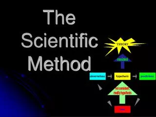
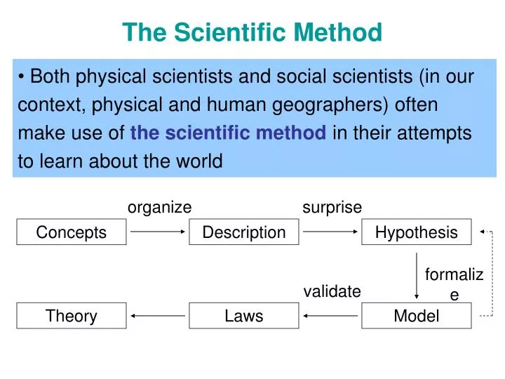
1. The Scientific Method organize surprise formalize validate • Both physical scientists and social scientists (in our context, physical and human geographers) often make use of the scientific method in their attempts to learn about the world Concepts Description Hypothesis Theory Laws Model

2. The Scientific Method • The scientific method gives us a means by which to approach the problems we wish to solve • The core of this method is the forming and testing of hypotheses • A very loose definition of hypotheses is potential answers to questions • Geographers use quantitative methods in the context of the scientific method in at least two distinct fashions:

3. organize surprise Concepts Description Hypothesis formalize validate Theory Laws Model Two Sorts of Approaches • Exploratory methods of analysis focus on generating and suggesting hypotheses • Confirmatorymethods are applied in order to test the utility and validity of hypotheses

4. Mathematical Notation • Summation Notation • Pi Notation • Factorial • Combinations

5. Two Sorts of Statistics • Descriptive statistics • To describe and summarize the characteristics of the sample • Fall within the class of exploratory techniques • Inferential statistics • To infer something about the population from the sample • Lie within the class of confirmatorymethods

6. Terminology • Population • A collection of items of interest in research • A complete set of things • A group that you wish to generalize your research to • An example – All the trees in Battle Park • Sample • A subset of a population • The size smaller than the size of a population • An example – 100 trees randomly selected from Battle Park

7. Terminology • Representative – An accurate reflection of the population (A primary problem in statistics) • Variables – The properties of a population that are to be measured (i.e., how do parts of the population differ? • Constant – Something that does not vary • Parameter – A constant measure which describes the characteristics of a population • Statistic – The corresponding measure for a sample

8. Descriptive Statistics • Descriptive statistics – Statistics that describe and summarize the characteristics of a dataset (sample or population) • Descriptive methods – Fall within the class of exploratory techniques • The most common way of describing a variable distribution is in terms of two of its properties: central tendency & dispersion

9. Descriptive Statistics • Measures of central tendency • Measures of the location of the middle or the center of a distribution • Mean, median, mode • Measures of dispersion • Describe how the observations are distributed • Variance, standard deviation, range, etc

10. Measures of Central Tendency – Mean • Mean – Most commonly used measure of central tendency • Average of all observations • The sum of all the scores divided by the number of scores • Note: Assuming that each observation is equally significant

11. Measures of Central Tendency – Mean Sample mean: Population mean:

12. Measures of Central Tendency – Mean • Example I • Data: 8, 4, 2, 6, 10 • Example II • Sample: 10 trees randomly selected from Battle Park • Diameter (inches): 9.8, 10.2, 10.1, 14.5, 17.5, 13.9, 20.0, 15.5, 7.8, 24.5

13. Measures of Central Tendency – Mean • Example III Annual mean temperature (°F) Monthly mean temperature (°F) at Chapel Hill, NC (2001).

14. Example IV Mean annual precipitation (mm) Mean 1198.10 (mm) Mean annual temperature ((°F) Mean 58.51 (°F) Chapel Hill, NC (1972-2001)

15. Measures of Central Tendency – Mean • Advantage • Sensitive to any change in the value of any observation • Disadvantage • Very sensitive to outliers Mean = 6.19 m Mean = 8.10 m Source: http://www.forestlearn.org/forests/refor.htm

16. Measures of Central Tendency – Mean • A standard geographic application of the mean is to locate the center (centroid) of a spatial distribution • Assign to each member a gridded coordinate and calculating the mean value in each coordinate direction --> Bivariate mean or mean center • For a set of (x, y) coordinates, the mean center is calculated as:

17. Map Coordinates • Geographic coordinates – The geographic coordinate system is a system used to locate points on the surface of the globe (degrees of latitude and longitude) • Geographic coordinates of Chapel Hill, NC • Lat: 35˚ 54’ 25’’N • Lon: 79˚ 02’ 55’’W Source: Xiao & Moody, 2004

18. Other map coordinates (UTM, state plane, Lambert, etc) • e.g., UTM (Universal Transverse Mercator) • Chapel Hill, NC  X: 676096.67 Y: 3975379.18 Source: http://shookweb.jpl.nasa.gov/validation/UTM/default.htm

19. Geographic Center of US (before 1959) Source: http://www.geocities.com/CapitolHill/Lobby/3162/HiPlains/GeoCenter/hiplains_geocenter.htm

20. Geographic Center of US (since 1959) • In 1959, after Alaska and Hawaii became states, the geographic center of the nation shifted far to the north and west of Lebanon KS • The geo-center is now located on private ranchland in a rural part of Butte County, SD Source: http://www.geocities.com/CapitolHill/Lobby/3162/HiPlains/GeoCenter50/

21. Shift of the Geographic Center of US

22. Shift of the Geographic Center of US Source: http://www.cia.gov/cia/publications/factbook/geos/us.html

23. Weighted Mean • We can also calculate a weighted mean using some weighting factor: e.g. What is the average income of all people in cities A, B, and C: CityAvg. IncomePopulation A $23,000 100,000 B $20,000 50,000 C $25,000 150,000 Here, population is the weighting factor and the average income is the variable of interest

24. Weighted Mean Center • We can also calculate a weighted mean center in much the same way, by using weights: For a set of (x, y) coordinates, the weighted mean center is computed as: e.g., suppose we had the centroids and areas of 3 polygons Here we weight by area

25. Example – Center of Population • Center of population reflects the spatial distribution of population • The shift of the center of population indicates the migration of population or changes in population over space • e.g., find the centroid and population of each state • The proportions of population can be used weights • Calculate the weighted mean

26. Center of Population Source: http://www.census.gov/geo/www/centers_pop.pdf

27. Shift of the Center of Population (1790 – 1950, 48 contiguous states)

28. Weighted Mean in Remote Sensing Source: http://rst.gsfc.nasa.gov/Sect13/Sect13_2.html

29. Weighted Mean in Remote Sensing About 850m IKONOS panchromatic image (2002-02-05)

30. Weighted Mean in Remote Sensing (Source: Lillesand et al. 2004) R is the signal (e.g., reflectance) for a given pixel fi is the proportion of each land surface type ri is the signal (e.g., reflectance) for each surface type N is the number of surface types

31. Measures of Central Tendency – Median • Median – This is the value of a variable such that half of the observations are above and half are below this value i.e. this value divides the distribution into two groups of equal size • When the number of observations is odd, the median is simply equal to the middle value • When the number of observations is even, we take the median to be the average of the two values in the middle of the distribution

32. Example I Data: 8, 4, 2, 6, 10 (mean: 6) Measures of Central Tendency – Median 2, 4, 6, 8, 10 median: 6 • Example II • Sample: 10 trees randomly selected from Battle Park • Diameter (inches): 9.8, 10.2, 10.1, 14.5, 17.5, 13.9, 20.0, 15.5, 7.8, 24.5 (mean: 14.38) 7.8, 9.8, 10.1, 10.2, 13.9, 14.5, 15.5, 17.5, 20.0, 24.5 median: (13.9 + 14.5) / 2 = 14.2

33. Mean = 6.19 m Mean = 8.10 m Source: http://www.forestlearn.org/forests/refor.htm median: (6.0 + 7.1) = 6.55 • Advantage: the value is NOT affected by extreme values at the end of a distribution (which are potentially are outliers)

34. Measures of Central Tendency – Mode • Mode - This is the most frequently occurring value in the distribution • This is the only measure of central tendency that can be used with nominal data • The mode allows the distribution's peak to be located quickly

35. Mean = 6.19 m (without outlier) Mean = 8.10 m Source: http://www.forestlearn.org/forests/refor.htm median: (6.0 + 7.1) = 6.55 mode: 7.5

36. Landsat ETM+, Chapel Hill (2002-05-24) (7-4-1 band combination) 24, 25, 30, 39, 40, 45, 45, 45, 45, 45, 48, 50, 50, 55, 58, 60, 61, 65, 65, 65, 70, 72, 75, 200, 205 mean: 63.28 median: 50 mode: 45 mean (without outliers): 51.17

37. Which one is better: mean, median, or mode? • Most often, the mean is selected by default • The mean's key advantage is that it is sensitive to any change in the value of any observation • The mean's disadvantage is that it is very sensitive to outliers • We really must consider the nature of the data, the distribution, and our goals to choose properly

38. Some Characteristics of Data • Not all data is the same. There are some limitations as to what can and cannot be done with a data set, depending on the characteristics of the data • Some key characteristics that must be considered are: • A. Continuous vs. Discrete • B. Grouped vs. Individual • C. Scale of Measurement

39. A. Continuous vs. Discrete Data • Continuous data can include any value (i.e., real numbers) • e.g., 1, 1.43, and 3.1415926 are all acceptable values. • Geographic examples: distance, tree height, amount of precipitation, etc • Discrete data only consists of discrete values, and the numbers in between those values are not defined (i.e., whole or integer numbers) • e.g., 1, 2, 3. • Geographic examples: # of vegetation types,

40. B. Grouped vs. Individual Data • The distinction between individual and grouped data is somewhat self-explanatory, but the issue pertains to the effects of grouping data • While a family income value is collected for each household (individual data), for the purpose of analysis it is transformed into a set of classes (e.g., <$10K, $10K-20K, > $20K) • e.g., elevation (1000m vs. < 500m, 500-1000m, 1000-2000m, > 2000m)

41. B. Grouped vs. Individual Data • In grouped data, the raw individual data is categorized into several classes, and then analyzed • The act of grouping the data, by taking the central value of each class, as well as the frequency of the class interval, and using those values to calculate a measure of central tendency has the potential to introduce a significant distortion • Grouping always reduces the amount of information contained in the data

42. C. Scales of Measurement • Data is the plural of a datum, which are generated by the recording of measurements • Measurements involves the categorization of an item (i.e., assigning an item to a set of types) when the measure is qualitative • or makes use of a number to give something a quantitative measurement

43. C. Scales of Measurement • The data used in statistical analyses can divided into four types: 1. The Nominal Scale 2. The Ordinal Scale 3. The interval Scale 4. The Ratio Scale As we progress through these scales, the types of data they describe have increasing information content

44. The Nominal Scale • Nominal scale data are data that can simply be broken down into categories, i.e., having to do with names or types • Dichotomous or binary nominal data has just two types, e.g., yes/no, female/male, is/is not, hot/cold, etc • Multichotomous data has more than two types, e.g., vegetation types, soil types, counties, eye color, etc • Not a scale in the sense that categories cannot be ranked or ordered (no greater/less than)

45. The Ordinal Scale • Ordinal scale data can be categorized AND can be placed in an order, i.e., categories that can be assigned a relative importance and can be ranked such that numerical category values have • star-system restaurant rankings 5 stars > 4 stars, 4 stars > 3 stars, 5 stars > 2 stars • BUT ordinal data still are not scalar in the sense that differences between categories do not have a quantitative meaning • i.e., a 5 star restaurant is not superior to a 4 star restaurant by the same amount as a 4 star restaurant is than a 3 star restaurant

46. The Interval Scale • Interval scale data take the notion of ranking items in order one step further, since the distance between adjacent points on the scale are equal • For instance, the Fahrenheit scale is an interval scale, since each degree is equal but there is no absolute zero point. • This means that although we can add and subtract degrees (100° is 10° warmer than 90°), we cannot multiply values or create ratios (100° is not twice as warm as 50°)

47. The Ratio Scale • Similar to the interval scale, but with the addition of having a meaningfulzero value, which allows us to compare values using multiplication and division operations, e.g., precipitation, weights, heights, etc • e.g., rain – We can say that 2 inches of rain is twice as much rain as 1 inch of rain because this is a ratio scale measurement • e.g., age – a 100-year old person is indeed twice as old as a 50-year old one

48. Which one is better: mean, median, or mode? • The mean is valid only for interval data or ratio data. • The median can be determined for ordinal data as well as interval and ratio data. • The mode can be used with nominal, ordinal, interval, and ratio data • Mode is the only measure of central tendency that can be used with nominal data

49. Which one is better: mean, median, or mode? • It also depends on the nature of the distribution Multi-modal distribution Unimodal symmetric Unimodal skewed Unimodal skewed

50. Which one is better: mean, median, or mode? • It also depends on your goals • Consider a company that has nine employees with salaries of 35,000 a year, and their supervisor makes 150,000 a year. • If you want to describe the typical salary in the company, which statistics will you use? • I will use mode or median (35,000), because it tells what salary mostpeople get Source: http://www.shodor.org/interactivate/discussions/sd1.html