Download
1 / 24
310 likes | 663 Views
9. Import Tariffs and Quotas under Imperfect Competition. Prepared by: Fernando Quijano Dickinson State University. 1 Tariffs and Quotas with Home Monopoly.

E N D
9 Import Tariffs and Quotas under Imperfect Competition Prepared by:Fernando Quijano Dickinson State University
1 Tariffs and Quotas with Home Monopoly • Tariffs and quotas affect the trade equilibrium differently because of their impact on the Home monopoly’s market power, the extent to which a firm can choose its price. • With a tariff, the Home monopolist still competes against a large number of importers, limiting its market power. • With a quota, once the quota is reached, the monopolist is the only producer able to sell in the Home market. The monopolist is again able to exercise its market power. • This section looks at Home equilibrium with and without trade, and explains the difference between tariffs and quotas.
1 Tariffs and Quotas with Home Monopoly No-Trade Equilibrium FIGURE 9-1 No-Trade Equilibrium In the absence of international trade, the monopoly equilibrium at Home occurs at the quantity QM, where marginal revenue equals marginal cost. From that quantity, we trace up to the demand curve at point A, and the price charged is PM. Under perfect competition, the industry supply curve is MC, so the no-trade equilibrium would occur where demand equals supply (point B), at the quantity QC and the price PC. Comparison with Perfect Competition In the absence of trade, the monopolist restricts its quantity sold to increase the market price. Under free trade, however, the monopolist cannot limit quantity and raise price.
1 Tariffs and Quotas with Home Monopoly Free-Trade Equilibrium FIGURE 9-2 (1 of 2) Home Monopoly’s Free-Trade Equilibrium Under free trade at the fixed world price PW, Home faces Foreign export supply of X*at that price. Because the Home firm cannot raise its price above PW without losing all of its customers to imports, X* is now also the demand curve faced by the Home monopolist. Because the price is fixed, the marginal revenue MR* is the same as the demand curve. Profits are maximized at point B, where marginal revenue equals marginal costs.
1 Tariffs and Quotas with Home Monopoly Free-Trade Equilibrium FIGURE 9-2 (2 of 2) Home Monopoly’s Free-Trade Equilibrium (continued) The Home firm supplies S1, and Home consumers demand D1. The difference between these is imports, M1 = D1 − S1. Because the Home monopoly now sets its price at marginal cost, the same free-trade equilibrium holds under perfect competition. Comparison with Perfect Competition Under free trade for a small country, then, a Home monopolist produces the same quantity and charges the same price as a perfectly competitive industry. The reason for this result is that free trade for a small country eliminates the monopolist’s control over price, that is, its market power.
1 Tariffs and Quotas with Home Monopoly Effect of a Home Tariff FIGURE 9-3 (1 of 2) Tariff with Home Monopoly Initially, under free trade at the fixed world price PW, the monopolist faces the horizontal demand curve (and marginal revenue curve) X*, and profits are maximized at point B. When a tariff t is imposed, the export supply curve shifts up since Foreign firms must charge PW + t in the Home market to earn PW. This allows the Home monopolist to increase its domestic price to PW + t, but no higher, since otherwise it would lose all of its customers to imports. Comparison with Perfect Competition Because the monopolist has limited control over its price, it behaves in the same way a competitive industry would when facing the tariff.
1 Tariffs and Quotas with Home Monopoly Effect of a Home Tariff FIGURE 9-3 (2 of 2) Tariff with Home Monopoly (continued) The result is fewer imports, M2, because Home supply S increases and Home demand D decreases. The deadweight loss of the tariff is measured by the area (b + d). This result is the same as would have been obtained under perfect competition because the Home monopolist is still charging a price equal to its marginal cost. Fall in consumer surplus: − (a + b + c + d) Rise in producer surplus: + a Rise in government revenue: + c Net effect on Home welfare: − (b + d) Home Loss Due to the Tariff
1 Tariffs and Quotas with Home Monopoly Effect of a Home Quota • Now we can look at the effect of a quota and compare it to the effect of a tariff. • The quota will end up with higher prices for Home consumers since it allows the monopolist to keep its market power, which we know leads to higher prices. • This is another reason why the WTO has encouraged countries to replace quotas with tariffs.
1 Tariffs and Quotas with Home Monopoly Effect of a Home Quota FIGURE 9-4 (1 of 2) Tariff with Home Monopoly Under free trade, the Home monopolist produces at point B and charges the world price of PW. With a tariff of t, the monopolist produces at point C and charges the price of PW + t. Imports under the tariff areM2 = D2 − S2. Under a quota of M2, the demand curve shifts to the left by that amount, resulting in the demand D − M2 faced by the Home monopolist. That is, after M2 units are imported, the monopolist is the only firm able to sell at Home, and so it can choose a price anywhere along the demand curve D – M2.
1 Tariffs and Quotas with Home Monopoly Effect of a Home Quota FIGURE 9-4 (2 of 2) Tariff with Home Monopoly (continued) The marginal revenue curve corresponding to D − M2 is MR, and so with a quota, the Home monopolist produces at point E, where MR equals MC. The price charged at point E is P3 > PW + t, so the quota leads to a higher Home price than the tariff. Home Loss Due to the Quota With an import quota, the Home firm is able to charge a higher price than it could with a tariff because it enjoys a “sheltered” market. So the import quota leads to higher costs for Home consumers than the tariff.
2 Tariffs with Foreign Monopoly Foreign Monopoly Free-Trade Equilibrium and Effect of a Tariff on Home Price FIGURE 9-7 (1 of 2) Tariff with a Foreign Monopoly Under free trade Foreign monopolist charges prices P1 and exports X1, where marginal revenue MR equals marginal cost MC*. When an antidumping duty of t is applied, the firm’s marginal cost rises to MC* + t, so the exports fall to X2 and the Home price rises to P2. The decrease in consumer surplus is shown by the area c + d, of which c is collected as a portion of tax revenues.
2 Tariffs with Foreign Monopoly Foreign Monopoly Free-Trade Equilibrium and Effect of a Tariff on Home Price FIGURE 9-7 (2 of 2) Tariff with a Foreign Monopoly Under free trade (continued) The net-of-tariff price that the Foreign exporter receives falls to P3 = P2 − t. Because the net-of-tariff price has fallen, the Home country has a terms-of-trade gain, area e. Thus, the total welfare change depends on the size of the terms-of-trade gain e relative to the deadweight loss d. Effect of the Tariff on Home Welfare Fall in Home consumer surplus: − (c + d) Rise in Home government surplus: + (c + e) Net change in Home welfare: + (e - d)
3 Dumping With international trade not only can firms charge a price that is higher than their marginal cost, they can also choose to charge different prices in their domestic market as compared with their export market. This pricing strategy is called price discrimination because the firm is able to choose how much different groups of customers pay.
3 Dumping Discriminating Monopoly We assume that the monopolist is able to charge different prices in the two markets; this market structure is sometimes called a discriminating monopoly. Equilibrium Condition For the discriminating monopoly, profits are maximized when the following condition holds:
3 Dumping FIGURE 9-8 (1 of 2) Foreign Discriminating Monopoly The Foreign monopoly faces different demand curves and charges different prices in its local and export markets. Locally, its demand curve is D* with marginal revenue MR*. Abroad, its demand curve is horizontal at the export price P, which is also its marginal revenue of MR. To maximize profits, the Foreign monopolist chooses to produce the quantity Q1at point B, where local marginal cost equals marginal revenue in the export market, MC* = MR.
3 Dumping FIGURE 9-8 (2 of 2) Foreign Discriminating Monopoly (continued) The quantity sold in the local market, Q2 (at point C), is determined where local marginal revenue equals export marginal revenue, MR* = MR. The Foreign monopolist sells Q2to its local market at P*, and Q1 –Q2 to its export market at P. Because P < P* (or alternatively P < AC1), the firm is dumping.
3 Dumping Numerical Example of Dumping
4 Policy Response to Dumping Antidumping Duties • Under the rules of the WTO, an importing country is entitled to apply an antidumping tariff any time that a foreign firm is dumping its product. • An imported product is being dumped if its price is below the price that the exporter charges in its own local market. • An example of an antidumping duty is the tariff that the European Union applies to imports of shoes from China and Vietnam. The European Union has also applied antidumping duty to Norwegian farmed salmon, but these were withdrawn after a WTO ruling
4 Policy Response to Dumping Calculation of Antidumping Duty FIGURE 9-9 (1 of 2) Home Loss Due to Threat of Duty A charge of dumping can sometimes lead Foreign firms to increase their prices, even without an antidumping duty being applied.
4 Policy Response to Dumping Calculation of Antidumping Duty FIGURE 9-9 (2 of 2) Home Loss Due to Threat of Duty (continued) In that case, there is a loss for Home consumers (a + b + c + d) and a gain for Home producers (a). The net loss for the Home country is area (b + c + d).
5 Infant Industry Protection • There are two cases in which infant industry protection is potentially justified. • First, protection may be justified if a tariff today leads to an increase in Home output that, in turn, helps the firm learn better production techniques and reduce costs in the future. • A second case in which import protection is potentially justified is when a tariff in one period leads to an increase in output and reductions in future costs for other firms in the industry, or even for firms in other industries. This type of externality occurs when firms learn from each other’s successes.
5 Infant Industry Protection In the semiconductor industry, it is not unusual for firms to mimic the successful innovations of other firms, and benefit from a knowledge spillover. As both of these cases show, the infant industry argument supporting tariffs or quotas depends on the existence of some form of market failure.
5 Infant Industry Protection Free-Trade Equilibrium and Tariff Equilibrium Equilibrium Today, Equilibrium in the Future, Effect of the Tariff on Welfare FIGURE 9-10 (1 of 2) Infant Industry Protection In the situation today (panel a), the industry would produce S1, the quantity at which MC = PW. Because PW is less than average costs at S1, the industry would incur losses at the world price of PW and would be forced to shut down. A tariff increases the price from PW to PW + t, allowing the industry to produce at S2 (and survive) with the net loss in welfare of (b + d).
5 Infant Industry Protection Free-Trade Equilibrium and Tariff Equilibrium Equilibrium Today, Equilibrium in the Future, Effect of the Tariff on Welfare FIGURE 9-10 (2 of 2) Infant Industry Protection (continued) In panel (b), producing today allows the average cost curve to fall through learning to AC. In the future, the firm can produce the quantity S3 at the price PW without tariff protection and earn producer surplus of e.