Download
1 / 22
220 likes | 366 Views
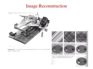
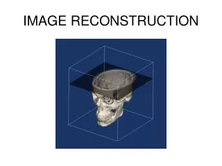
Tomographic Image Reconstruction Using Content-Adaptive Mesh Modeling. H. Can Aras November 29-30, 2004 Project Presentation. Reconstruction of CT-Images from Projection Data. Content-Adaptive Mesh Generation Estimation of Mesh Nodal Values Reconstruction of the Image by Interpolation.

E N D
Tomographic Image Reconstruction Using Content-Adaptive Mesh Modeling H. Can Aras November 29-30, 2004 Project Presentation
Reconstruction of CT-Images from Projection Data Content-Adaptive Mesh Generation Estimation of Mesh Nodal Values Reconstruction of the Image by Interpolation Problem Approach
Feature Map Extraction • Second derivative used, below is the theoretical basis for this. • M2 : the least upper bound on the second directional derivative of f(x) over T • h : the length of the longest side of T • The formula tells us two things…
Feature Map Extraction (cont.) To achieve a low approximation error of the image: • Small elements in large second derivative regions • Relatively larger elements in relatively small derivative regions
Feature Map Extraction (cont.) • Not practical to calculate directional derivatives • Use max (| fxx |, | fxy |, | fyy |) or the magnitude of the second derivative • Normalization of feature map • Segmentation of heart and background region • Modification of feature map
Placement of Mesh Nodes • Floyd-Steinberg error-diffusion algorithm • Originally designed for digital halftoning • The objective is to use the spatial density of the ink dots to represent the image intensity. • The classical method used varying ink dot sizes.
Placement of Mesh Nodes (cont) • Distribute errors among pixels • Uses the perception characteristics of the human eye • Fast, efficient and produces excellent results (almost)
Connecting Mesh Nodes • Delaunay triangulation • Returns set of triangles such that no data point is contained in any triangle’s circumcircle • Known to yield a well-structured mesh • Avoids producing excessively elongated elements, reducing the error bound
Reconstruction of Image • Pixel value is approximated from the nodal values of its enclosing triangle • Master element • Shape functions
Numerical Comparison • PSNR of FBP result : 47.51 • PSNR of MESH-ML result: 46.77 • compression rate: 5.36 • Note: A higher PSNR does not always correlate well with the perceived image quality (although it provides a measure for relative quality) • A slight change on MESH-ML result gives higher PSNR. • Subtracting only 0.01 from each value of MESH-ML result yields a PSNR of 48.81. Subtracting 0.02 yields 51.05! • The authors may be using another trick for PSNR!
A Comment on Results • The mesh nodal values tend to increase slightly on average after MESH-ML. • Until a number of iterations, the results get better. Behind this limit, results tend to go bad, even worse than FBP (reference) image.
Problems Faced • Radon Transform followed by Inverse Radon Transform yielded an image with negative values because of incomplete set of projections. • I adjusted this image between [0,1] so that the initial values of the mesh nodes are not negative in MESH-ML algorithm.
Problems Faced (cont.) • Delaunay Triangulation is sensitive to the position of the nodes. • Degenerate cases occur frequently when using integers for position coordinates. • I randomly changed the position coordinates with very small differences and used double instead of integer.
Problems Faced (cont.) • The analytical form of the response function is not known. • Hence, I calculated the system matrix by probing the input with an impulse function as offered in the paper. • Specifically, a unit-impulse was applied at each nodal location of the mesh model, and the response at each detector was computed. • This computation is time and memory consuming. • Time problem can be overcome by precalculation. • I used sparse matrix since most of the system matrix is zeros. • The MESH-ML algorithm takes longer than expected.
Plan • Try to make MESH-ML algorithm faster (not the main concern, but can be a bottle-neck for the tests below). • Run MESH-ML with multiple iterations. • Use better reference image in terms of the number of projection angles (5 degrees used between consecutive projections in the experiments). • Use better reference image in terms of the filter used in Fourier domain (Ram-Lak ramp filter used in the experiments). • Test on medical images, which capture different parts of the body.
Thank you for listening… Wish me more luck!