Download
1 / 43
440 likes | 520 Views
Lecture 5 Ideal Gases of Bosons and Fermions. Dhani Herdiwijaya v1.0. We have considered systems with a fixed number of particles at low particle densities , n << n Q . We allowed these systems to exchange only energy with the environment/reservoir

E N D
Lecture 5Ideal Gases of Bosons and Fermions Dhani Herdiwijaya v1.0
We have considered systems with a fixed number of particles at low particle densities, n<<nQ. We allowed these systems to exchange only energy with the environment/reservoir Now, we’ll remove both constraints: (a) we’ll extend our analysis to the case where both energy and matter can be exchanged (grand canonical ensemble), and (b) we’ll consider arbitrary n (quantum statistics). When we consider systems that can exchange particles and energy with a large reservoir, both and T are dictated by the reservoir (they are the reservoir’s properties). In particular, the equilibrium is reached when the chemical potentials of a system and its environment become equal to one another. In equilibrium, there is no net mass transfer, though the number of particles in a system can fluctuate around its mean value (diffusive equilibrium).
For a system with a fixed number of particles, we found that the probability P(i) of finding the system in the state with a particular energy i is given by the canonical distribution: We want to generalize this result to the case where both energy and particles can be exchanged with the environment.
From Particle States to Occupation Numbers Systems with a fixed number of particles in contact with the reservoir, occupancy ni<<1 Systems which can exchange both energy and particles with a reservoir, arbitrary occupancy ni 4 4 3 3 2 2 1 1 The energy was fluctuating, but the total number of particles was fixed. The role of the thermal reservoir was to fix the mean energy of each particle (i.e., each system). The identical systems in contact with the reservoir constitute the canonical ensemble. This approach works well for the high-temperature (classical) case, which corresponds to the occupation numbers <<1. When the occupation numbers are ~ 1, it is to our advantage to choose, instead of particles, a single quantum level as the system, with all particles that might occupy this state. Each energy level is considered as a sub-system in equilibrium with the reservoir, and each level is populated from a particle reservoir independently of the other levels.
From Particle States to Occupation Numbers (cont.) We will consider a system of identical non-interacting particles at the temperature T, i is the energy of a single particle in the i state, ni is the occupation number (the occupancy) for this state: The energy of the system in the state s {n1, n2, n3,.....} is: The grand partition function: The sum is taken over all possible occupancies and all states for each occupancy. The Gibbs sum depends on the single-particle spectrum (i), the chemical potential, the temperature, and the occupancy. The latter, in its tern, depends on the nature of particles that compose a system (fermions or bosons). Thus, in order to treat the ideall gas of quantum particles at not-so-small ni, we need the explicit formulae for ’s and nifor bosons and fermions.
Spin of elementary particles • Elementary particles are particles that cannot be divided into any smaller units, such as the photon, the electron, and the various quarks. • Theoretical and experimental studies have shown that the spin possessed by these particles cannot be explained by postulating that they are made up of even smaller particles rotating about a common center of mass (see classical electron radius); as far as can be determined, these elementary particles are true point particles. • The spin that they carry is a truly intrinsic physical property, akin to a particle's electric charge and mass.
Spin of elementary particles • In quantum mechanics, the angular momentum of any system is quantized: its magnitude can only take values • where h is the reduced Planck's constant, and the spin quantum numbers is a non-negative integer or half-integer (0, 1/2, 1, 3/2, 2, etc.). The possibility of half-integer quantum numbers is a major difference between spin and orbital angular momentum; the latter can only take integer quantum numbers. The value of s depends only on the type of particle, and cannot be altered in any known way (in contrast to the spin direction). • For instance, all electrons have s = 1/2. Other elementary spin-1/2 particles include positrons, neutrinos and quarks. Photons are spin-1 particles, and the hypothetical graviton is a spin-2 particle. The hypothetical Higgs boson is unique among elementary particles in having a spin of zero.
Satyendra Nath Bose (1894 –1974) and Albert Einstein (1879 – 1955) B-E statistics was introduced for photons in 1920 by Bose and generalized to atoms by Einstein in 1924
History • In the early 1920s Satyendra Nath Bose , a professor of University of Dhaka was intrigued by Einstein's theory of light waves being made of particles called photons. Bose was interested in deriving Planck's radiation formula, which Planck obtained largely by guessing. • In 1900 Max Planck had derived his formula by manipulating the math to fit the empirical evidence. Using the particle picture of Einstein, Bose was able to derive the radiation formula by systematically developing a statistics of massless particles without the constraint of particle number conservation.
History • Bose derived Planck's Law of Radiation by proposing different states for the photon. Instead of statistical independence of particles, Bose put particles into cells and described statistical independence of cells of phase space. Such systems allow two polarization states, and exhibit totally symmetric wave-functions. • He developed a statistical law governing the behavior pattern of photons quite successfully. However, he was not able to publish his work; no journals in Europe would accept his paper, being unable to understand it. Bose sent his paper to Einstein, who saw the significance of it and used his influence to get it published.
Boson particles In particle physics, bosons are particles which obey Bose-Einstein statistics; they are named after Satyendra Nath Bose and Albert Einstein. In contrast to fermions, which obey Fermi-Dirac statistics, after Enrico Fermi and Paul Dirac Several bosons can occupy the same quantum state. Thus, bosons with the same energy can occupy the same place in space. Therefore bosons are often force carrier particles while fermions are usually associated with matter. Bosons may be either elementary, like the photon, or composite, like mesons. All observed bosons have integer spin, as opposed to fermions, which have half-integer spin.
Bosons and Fermions One of the fundamental results of quantum mechanics is that all particles can be classified into two groups. Bosons: particles with zero or integer spin (in units of ħ). Examples: photons, all nuclei with even mass numbers. The wavefunction of a system of bosons is symmetric under the exchange of any pair of particles: (...,Qj,...Qi,..)= (...,Qi,...Qj,..). The number of bosons in a given state is unlimited. Fermions: particles with half-integer spin (e.g., electrons, proton, all nuclei with odd mass numbers); the wavefunction of a system of fermions is anti-symmetric under the exchange of any pair of particles: (...,Qj,...Qi,..)= -(...,Qi,...Qj,..). The number of fermions in a given state is zeroor one (the Pauli exclusion principle).
Bosons and Fermions The Bose or Fermi character of composite objects: the composite objects that have even number of fermions are bosons and those containing an odd number of fermions are themselves fermions. (an atom of 3He = 2 electrons + 2 protons + 1 neutron hence 3He atom is a fermion) In general, if a neutral atom contains an odd # of neutrons then it is a fermion, and if it contains en even # of neutrons then it is a boson. The difference between fermions and bosons is specified by the possible values of ni: fermions:ni= 0 or 1 bosons: ni= 0, 1, 2, .....
Fermion Boson Particle physics mass charge spin name
Boson Particles Most bosons are composite particles, in the Standard Model, there are five bosons which are elementary: • the gauge bosons, e.g γ (photon) · g (gluon) · W± · Z (W&Z boson); • the Higgs boson (H0). Unlike the gauge bosons, the Higgs boson has not yet been observed experimentally. The Standard Model of particle physics is a theory of three of the four known fundamental interactions and the elementary particles that take part in these interactions. These particles make up all visible matter in the universe. The Standard Model falls short of being a complete theory of fundamental interactions because it does not include gravity and because it is incompatible with the recent observation of neutrino oscillations.
The Partition Function of an Ideal Bose Gas The grand partition function for all particles in the ith single-particle state: (the sum is taken over the possible values of ni) If the particles are bosons, n can any integer 0: - the partition function for the Bose-Einstein gas
Bose-Einstein Distribution The mean number of bosons in a given state: The Bose-Einstein distribution
2 BE FD 1 = 0 BE and FD The mean number of particles in a given state for the BEG can exceed unity, it diverges as . Comparison of the FD and BE distributions plotted for the same value of .
Enrico Fermi(1901 – 1954)and Paul Adrien Maurice Dirac (1902-1984) There are two possible outcomes: If the result confirms the hypothesis, then you've made a measurement. If the result is contrary to the hypothesis, then you've made a discovery.
History • Before the introduction of Fermi–Dirac statistics in 1926, understanding some aspects of electron behavior was difficult due to seemingly contradictory phenomena. • It was difficult to understand, why electrons in a metal can move freely to conduct electric current, while their contribution in the same metal to the specific heat was negligible, as if there were considerably fewer electrons. • It was also difficult to understand why the emission currents, generated by applying high electric fields to metals at room temperature, were almost independent of temperature. • The difficulty encountered by the electronic theory of metals at that time was due to considering that electrons were (according to classical statistics theory) all equivalent. In other words it was believed that each electron contributed to the specific heat an amount of the order of the Boltzmann constant k. This statistical problem remained unsolved until the discovery of F–D statistics.
History • F–D statistics was first published in 1926 by Enrico Fermi and Paul Dirac. According to an account, Pascual Jordan developed in 1925 the same statistics which he called Pauli statistics, but it wasn't published in a timely manner. Whereas according to Dirac, it was first studied by Fermi, and Dirac called it Fermi statistics and the corresponding particles fermions. • F–D statistics was applied in 1926 by Fowler to describe the collapse of a star to a white dwarf. • In 1927 Sommerfeld applied it to electrons in metals • In 1928 Fowler and Nordheim applied it to field electron emission from metals. • Fermi–Dirac statistics continues to be an important part of physics.
Fermion particles The known elementary fermions are divided into two groups: quarks and leptons. • Quarks make up protons, neutrons and other baryons, which are composite fermions; they also comprise mesons, which are composite bosons. • Leptons include the electron and similar, heavier particles (the muon and tauon); they also include neutrinos. The known fermions of left-handed helicity experience weak interactions while the known right-handed fermions do not. Or put another way, only left-handed fermions and right-handed anti-fermions interact with the W boson.
The Partition Function of an Ideal Fermi Gas A system that consists of just one singlestate of energy i. The total energy of this state: ni i. The probability of this state to be occupied by ni particles: The grand partition function for all particles in the ith single-particle state (the sum is taken over all possible values of ni) : If the particles are fermions, n can only be 0 or 1: the full partition function is given by:
1 The partition functions of different levels are multiplied because they are independent of one another (each level is an independent thermal system, it is filled by the reservoir independently of all other levels).
Fermi-Dirac Distribution The probability of a state to be occupied by a fermion: The mean number of fermions in a particular state: - the Fermi-Dirac distribution ( is determined by T and the particle density)
1 ~ kBT T=0 0 = (with respect to) At T = 0, all the states with < have the occupancy = 1, all the states with > have the occupancy = 0 (i.e., they are unoccupied). With increasing T, the step-like function is “smeared” over the energy range ~ kBT. The macrostate of such system is completely defined if we know the mean occupancy for all energy levels, which is often called the distribution function: n=N/V – the average density of particles While f(E) is often less than unity, it is not a probability:
Classical limit For sufficiently largewe will have (-)/kT>>1, and in this limit This is just the Boltzmann distribution. The high-energy tail of the Fermi-Dirac distribution is similar to the Boltzmann distribution. The condition for the approximate validity of the Boltzmann distribution for all energies 0is that
Distribusi Fermi-Dirac Energy dependence. More gradual at higher T. μ decreases for higher T Temperature dependence for ε>μ .
The Classical Regime Comparison of the FD and BE distributions plotted for the same value of . Note that the MB distribution makes no sense when the average # of particle in a given state becomes comparable to 1 (violation of the classical limit). 2 MB BE FD 1 = 0 The FD and BE distributions are reduced to the Boltzmann distribution in the classical limit: - this is still not the Boltzmann factor: we deal with the -fixed formalism whereas the Boltzmann factor is the distribution function in the N-fixed formalism.
To get to the N-fixed formalism, let’s add all nk for all single-particle states and demand that be such that the total number of occupancies is equal to N: This is consistent with our initial assumption that The resulting chemical potential is the same as what we obtained in the classical regime:
The Classical Regime (cont.) The free energy in the classical regime: The chemical potential of Boltzmann gas (the classical regime): μ for an ideal gas is negative: when you add a particle to a system and want to keep Sfixed, you typically have to remove some energy from the system.
In terms of the density, the classical limit corresponds to n << nQ (quantum density): We can also rewrite this condition as T>>TC where TC is the so-called degeneracy temperature of the gas, which corresponds to the condition n~ nQ. More accurately: For the FD gas, TC ~ EF/kB where EFis the Fermi energy, for the BE gas TC is the temperature of BE condensation
/EF n ~ nQ 1 kBT/EF 1 for Fermi Gases When the average number of fermions in a system (their density) is known, this equation can be considered as an implicit integral equation for (T,n). It also shows that determines the mean number of particles in the system just as T determines the mean energy. However, solving the eq. is a non-trivial task. depending on n and T, for fermions may be either positive or negative.
The limit T0: adding one fermion to the system at T=0 increases its energy U by EF. At the same time, S remains0: all the fermions are packed into the lowest-energy states.
The same conclusion you’ll reach by considering F=U-TS=UT=0 and recalling that the chemical potential is the change in F produced by the addition of one particle: The change of sign of (n,T) indicates the crossover from the degenerate Fermi system (low T, high n) to the Boltzmann statistics. The condition kBT << EF is equivalent to n >> nQ:
T for Bose Gases Bose Gas The occupancy cannot be negative for any , thus, for bosons, 0 ( varies from 0 to ). Also, as T0, 0 For bosons, the chemical potential is a non-trivial function of the density and temperature (for details, see the lecture on BE condensation
3 2 1 1 2 3 Comparison between Distributions Fermi-Dirac Boltzmann Bose-Einstein 3 2 zero-point energy, Pauli principle 1 1 2 3
Comparison between Distributions CV /NkB Fermi-Dirac Boltzmann Bose-Einstein 2 1.5 0 1 T/TC
Comparison between Distributions Bose Einstein Fermi Dirac Boltzmann • indistinguishable • half-integer spin 1/2,3/2,5/2 … • fermions • wavefunctions overlap total anti-symmetric free electrons in metals electrons in white dwarfs never more than 1 particle per state • indistinguishable • Z=(Z1)N/N! • nK<<1 • spin doesn’t matter • localized particles don’t overlap gas molecules at low densities “unlimited” number of particles per state • nK<<1 • indistinguishable • integer spin 0,1,2 … • bosons • wavefunctions overlap total symmetric photons 4He atoms unlimited number of particles per state
Problem (partition function, fermions) Calculate the partition function of an ideal gas of N=3 identical fermions in equilibrium with a thermal reservoir at temperature T. Assume that each particle can be in one of four possible states with energies 1, 2, 3, and 4. (Note that N is fixed). The Pauli exclusion principle leaves only four accessible states for such system. (The spin degeneracy is neglected). the number of particles in the single-particle state The partition function: the system is in a state with Ei Calculate the grand partition function of an ideal gas of fermions in equilibrium with a thermal and particle reservoir (T, ). Fermions can be in one of four possible states with energies 1, 2, 3, and 4. (Note that N is not fixed). 4 3 2 each level I is a sub-system independently “filled” by the reservoir 1