Download

1 / 29
300 likes | 421 Views
This seminar explores the development of parallel algorithms for tackling geometric graph problems, emphasizing efficient approximation techniques in time and space. In particular, we focus on properties such as linear and sublinear running times, which are crucial for managing big data in computational settings. Key algorithms and methodologies are examined, covering foundational work from the 1930s to modern advancements, highlighting the applicability of combinatorial methods in a parallel computational framework. Join us to delve into the future of algorithmic theory in the context of massive parallelization.

E N D
Parallel Algorithms for Geometric Graph Problems GrigoryYaroslavtsev 361 Levine http://grigory.us STOC 2014, joint work with AlexandrAndoni, Krzysztof Onak and AleksandarNikolov.
Theory Seminar: Fall 14 • Fridays 12pm1pm • 512 Levine / 612 Levine • Homepage: http://theory.cis.upenn.edu/seminar/ • Google Calendar: see link above • Announcements: • Theory list: http://lists.seas.upenn.edu/mailman/listinfo/theory-group
“The Big Bang Data Theory” What should TCS say about big data? • Usually: • Running time: (almost) linear, sublinear, … • Space: linear, sublinear, … • Approximation: best possible, … • Randomness: as little as possible, … • Special focus today: roundcomplexity
Round Complexity Information-theoretic measure of performance • Tools from information theory (Shannon’48) • Unconditional results (lower bounds) Example today: • Approximating Geometric Graph Problems
Approximation in Graphs 1930-50s: Given a graph and an optimization problem… Minimum Cut(RAND): Harris and Ross [1955] (declassified, 1999) Transportation Problem: Tolstoi [1930]
Approximation in Graphs 1960s: Single processor, main memory (IBM 360)
Approximation in Graphs 1970s: NP-complete problem – hard to solve exactly in time polynomial in the input size “Black Book”
Approximation in Graphs Approximate with multiplicative error on the worst-case graph : Generic methods: • Linear programming • Semidefiniteprogramming • Hierarchies of linear and semidefinite programs • Sum-of-squares hierarchies • …
The New: Approximating Geometric Problems in Parallel Models 1930-70s to 2014
The New: Approximating Geometric Problems in Parallel Models Geometric graph (implicit): Euclidean distances betweennpoints in Already have solutions for old NP-hard problems (Traveling Salesman, Steiner Tree, etc.) • Minimum Spanning Tree (clustering, vision) • Minimum Cost Bichromatic Matching (vision)
Geometric Graph Problems Combinatorial problems on graphs in Polynomial time(“easy”) • Minimum Spanning Tree • Earth-Mover Distance = Min Weight Bi-chromatic Matching NP-hard(“hard”) • Steiner Tree • Traveling Salesman • Clustering (k-medians, facility location, etc.) Need new theory! Arora-Mitchell-style “Divide and Conquer”, easy to implement in Massively Parallel Computational Models
MST: Single Linkage Clustering • [Zahn’71] Clustering via MST (Single-linkage): kclusters: remove longest edges from MST • Maximizes minimumintercluster distance [Kleinberg, Tardos]
Earth-Mover Distance • Computer vision: compare two pictures of moving objects (stars, MRI scans)
Computational Model • Input: npoints in a d-dimensional space (d constant) • machines, space on each ( = , ) • Constant overhead in total space: • Output: solution to a geometric problem (size O() • Doesn’t fit on a single machine () points ⇒ machines S space
Computational Model • Computation/Communication in rounds: • Every machine performs a near-linear timecomputation => Total running time • Every machine sends/receives at most bits of information => Total communication . Goal:Minimize . Our work: = constant. bits machines time S space
MapReduce-style computations What I won’t discuss today • PRAMs (shared memory, multiple processors) (see e.g. [Karloff, Suri, Vassilvitskii‘10]) • Computing XOR requires rounds in CRCW PRAM • Can be done in rounds of MapReduce • Pregel-style systems, Distributed Hash Tables (see e.g. Ashish Goel’s class notes and papers) • Lower-level implementation details (see e.g. Rajaraman-Leskovec-Ullman book)
Models of parallel computation • Bulk-Synchronous Parallel Model (BSP) [Valiant,90] Pro: Most general, generalizes all other models Con: Many parameters, hard to design algorithms • Massive Parallel Computation[Feldman-Muthukrishnan-Sidiropoulos-Stein-Svitkina’07, Karloff-Suri-Vassilvitskii’10, Goodrich-Sitchinava-Zhang’11, ..., Beame, Koutris, Suciu’13] Pros: • Inspired by modern systems (Hadoop, MapReduce, Dryad, … ) • Few parameters, simple to design algorithms • New algorithmic ideas, robust to the exact model specification • # Rounds is an information-theoretic measure => can prove unconditional lower bounds • Between linear sketching and streaming with sorting
Previous work • Dense graphs vs. sparse graphs • Dense: (or solution size) “Filtering” (Output fits on a single machine) [Karloff, SuriVassilvitskii, SODA’10; Ene, Im, Moseley, KDD’11; Lattanzi, Moseley, Suri, Vassilvitskii, SPAA’11; Suri, Vassilvitskii, WWW’11] • Sparse: (or solution size) Sparse graph problems appear hard (Big open question: (s,t)-connectivity in rounds?) VS.
Large geometric graphs • Graph algorithms: Dense graphs vs. sparse graphs • Dense: . • Sparse: . • Our setting: • Dense graphs, sparsely represented: O(n) space • Output doesn’t fit on one machine () • Today: -approximate MST • (easy to generalize) • rounds ()
-MST inrounds • Assume points have integer coordinates , where Impose an -depth quadtree Bottom-up: For each cell in the quadtree • compute optimum MSTs in subcells • Use only onerepresentativefrom each cell on the next level Wrong representative: O(1)-approximation per level
-nets • -net for a cell C with side length : Collection S of vertices in C, every vertex is at distance <= from some vertex in S. (Fact: Can efficiently compute -net of size Bottom-up: For each cell in the quadtree • Compute optimum MSTs in subcells • Use -net from each cell on the next level • Idea: Pay only ) for an edge cut by cell with side • Randomly shift the quadtree: – charge errors Wrong representative: O(1)-approximation per level
Top cell shifted by a random vector in Impose a randomly shiftedquadtree(top cell length ) Bottom-up: For each cell in the quadtree • Compute optimum MSTs in subcells • Use -net from each cell on the next level Pay 5 instead of 4 Pr[] = (1) 2 1
-MST inrounds • Idea: Only use short edges inside the cells Impose a randomly shiftedquadtree(top cell length ) Bottom-up: For each node (cell) in the quadtree • compute optimum Minimum Spanning Forestsin subcells, using edges of length • Use only -net from each cell on the next level Sketch of analysis ( = optimum MST): 𝔼[Extra cost] = 𝔼 2 Pr[] = 1
-MST inrounds • rounds => O() = O(1) rounds • Flatten the tree: ()-grids instead of (2x2) grids at each level. Impose a randomly shifted ()-tree Bottom-up: For each node (cell) in the tree • compute optimum MSTs in subcellsvia edges of length • Use only -net from each cell on the next level ⇒
-MST inrounds Theorem: Let = # levels in a random tree P Proof (sketch): • = cell length, which first partitions • New weights: • Our algorithm implements Kruskalfor weights
“Solve-And-Sketch” Framework -MST: • “Load balancing”: partition the tree into parts of the same size • Almost linear time: Approximate Nearest Neighbor data structure [Indyk’99] • Dependence on dimension d (size of -net is • Generalizes to bounded doubling dimension • Basic version is teachable (Jelani Nelson’s ``Big Data’’ class at Harvard) • Implementation in progress…
“Solve-And-Sketch” Framework -Earth-Mover Distance, Transportation Cost • No simple “divide-and-conquer” Arora-Mitchell-style algorithm (unlike for general matching) • Only recently sequential -apprxoimation in time [Sharathkumar, Agarwal ‘12] Our approach (convex sketching): • Switch to the flow-based version • In every cell, send the flow to the closest net-point until we can connect the net points
“Solve-And-Sketch” Framework Convex sketching the cost function for net points • = the cost of routing fixed amounts of flow through the net points • Function “normalization” is monotone, convex and Lipschitz, ()-approximates • We can ()-sketch it using a lower convex hull
Thank you!http://grigory.us Open problems: • Exetension to high dimensions? • Probably no, reduce from connectivity => conditional lower bound rounds for MST in • The difficult setting is (can do JL) • Streaming alg for EMD and Transporation Cost? • Our work: • First near-linear time algorithm for Transportation Cost • Is it possible to reconstruct the solution itself?