Download
1 / 23
230 likes | 370 Views
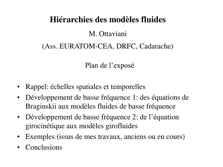
Hiérarchies des modèles fluides M. Ottaviani (Ass. EURATOM-CEA, DRFC, Cadarache). Plan de l’exposé Rappel: échelles spatiales et temporelles Développement de basse fréquence 1: des équations de Braginskii aux modèles fluides de basse fréquence

E N D
Hiérarchies des modèles fluidesM. Ottaviani(Ass. EURATOM-CEA, DRFC, Cadarache) Plan de l’exposé • Rappel: échelles spatiales et temporelles • Développement de basse fréquence 1: des équations de Braginskii aux modèles fluides de basse fréquence • Développement de basse fréquence 2: de l’équation girocinétique aux modèles girofluides • Exemples (issus de mes travaux, anciens ou en cours) • Conclusions
From kinetic to fluid: classical approach • Kinetic equation (collision dominated) ==> • Chapman-Enskog expansion ==> • Braginskii equations (1960) ==> • low frequency expansions (drift ordering) ==> • models, eventually ad hoc closures
From kinetic to fluid: gyrofluid approach (since 1990) • Kinetic equation, non collisional (Vlasov) ==> • low frequency expansion ==> • gyrokinetic equation ==> • moments, closures ==> • hierarchy of gyrofluid models
Example 1. Collisionless reconnection: sawtooth crash Result (Ottaviani & Porcelli, 1993) Current sheet formation on a fast timescale, controlled by el. inertia.
Example 2. Tearing-modes at low collisionality • Analysis of tearing modes (reconnecting modes) in regimes of low collisionality. The drift frequency exceeds the collision frequency. Electron inertia comes into play • Employs the four-field model • Study linear stability criteria. • Search for bistability (coexistence of states). • Coupling to drift waves Electrostatic solution, small island de-localized electric potential, drift-wave Electromagnetic solution, island localized electric potential
Example 3. Ion temperature gradient turbulence • General goal: determine the dependence of turbulent thermal transport as a function of dimensionless parameters (Manfredi & Ottaviani, 1997, and foll.) • ITG model:
Conclusions (personal) • Conventional low frequency fluid models still useful, at least for a first approach to a given problem • Gyrofluid models more flexibles, take naturally into account the anisotropy • Good practical closures for the parallel dynamics exist, if sufficiently high order momenta are kept, especially when magnetic fluctiations are present • FLR closures still involved, complicated. Problematic at very short wavelengths (below the ion Larmor radius) • More work ?