Download
1 / 25
250 likes | 395 Views
Critical remarks on. Wells et al., Motorcycle rider conspicuity... October 26, 2009 Jørgen Hilden j.hilden@biostat.ku.dk. This is a marvelous study – esp. considering costs Unfortunately it is somewhat undersized Notes have been added in this PowerPoint file.

E N D
Critical remarks on Wells et al., Motorcycle rider conspicuity... October 26, 2009 Jørgen Hilden j.hilden@biostat.ku.dk
This is a marvelous study – esp. considering costsUnfortunately it issomewhat undersized Notes have been added in this PowerPoint file
Critique Night-time experience not reported “as less than 2% af the riding … ” (How many percent of the accidents?, I would ask.) It appears that the authors believe that risk can only depend on the front of the rider.
Case-control philosophy Theoretical aside Incidence: events are 2.5 times as frequent in periods of exposure Same with a non-repeatable event (mortality, melanoma diagnosis) Prevalence, determined to be 25% via a randomly placed snapshot (”cross-sectional study”) a ’life line’
Case-control philosophy Theoretical aside Incidence: events are 2.5 times as frequent in period of exposure Same with non-repeatable event (mortality, melanoma diagnosis) Prevalence of exposure determined via a randomly placed snapshot (”cross-sectional study”) Control data: Time accumulated (= ” optjent ”) in each exposure group is apportioned by means of a snapshot of the population. Put simply, a randomly placed snapshort imitates [when properly done] the occurrence pattern of a type of event (’control event’) that has an exposure-independent incidence rate. – ORs then give the desired incidence ratios.
Case-control philosophy Theoretical aside Variants Cases = snapshot of schizophrenic population Controls = general school files ?: problematic behaviour in school or not? Research question: does problem behaviour predispose to time spent with your schizophrenia diagnosis (once you get it)? - - - - - - Cases = snapshot of patients out of work after tibial fracture Controls = ’incident’ tibial fracture events ? : was it a MC accident? Research question concerns duration: do tibial fractures that are due to MC accidents show particularly slow healing? [ Here the roles of snapshots and event examination are reversed compared with ’normal’ C-C studies. ]
Case-control philosophy:What would be the ideal control sampling for (driver-related) motorcycle accidents? Let’s ask: (1) What data would an omniscient but non-interfering God collect? – And (2) can we regard Wells’s actual control scheme as a reasonable approximation to that? A two-step plan
What data would an omniscient but non-interfering God collect? • ? An angel’s-view snapshot of all MC drivers on Auckland roads at the moment the accident occurred – • possibly with restrictions as to local characteristics (type of road, local wetness, etc.)
What data would an omniscient but non-interfering God collect? • ? An angel’s-view snapshot of all MC drivers on Auckland roads at the moment the accident occurred – • possibly with restrictions as to local characteristics (type of road, local wetness, etc.) NO!
What data would an omniscient but non-interfering God collect? • ? An angel’s-view snapshot of all MC drivers on Auckland roads at the moment the accident occurred – • possibly with restrictions as to local characteristics (type of road, local wetness, etc.) NO! That would make it an incidence rate study (accident risk per hour on bike)
What data would an omniscient but non-interfering God collect? No, we want the risk per km travelled and that requires a roadside control sampling (Wells!): if that is correctly done, the chance of being stopped for an interview is proportional to distance travelled. Proof: think of the God placing an interviewer for every 100 m at all times – and subject this ideal design to independent random thinning. I assume focus on ’risk per km’ and not, e.g., ’risk per intersection passed’
What data would an omniscient but non-interfering God collect? Note: this has nothing to do with whether fast driving is more or less dangerous per km than slow driving. You must simply realize that: Random time controls accident risk per time unit. Which we don’t want. Random location control accident risk per Δlocation (i.e., per km of mileage).
in other words Random location control risk per Δlocation [km of mileage] Events are 2.5 times as dense in street sections (or meters of travel) under exposure A randomly placed streetshot (a literally cross-sectional study!) shows that 25% of mileage is travelled under exposure. a road line
Grafisk køreplan What data would an omniscient but non-interfering God collect? One fast and one slow hourly train run from Kbh. to Korsør. At the time of the accident 08:42 fast control trains are under- represented. Sampling at the location (west of Roskilde) will reflect the true mix of trains. Accident
(2) Can we regard Wells’s actual control scheme as a reasonable approximation? ”We randomly selected these sites from a list of all non-residential roads in the region, in proportion to their total length.” Acceptable! – even considering Avs. B: to city A B Cul de sac
A Lorenz curve The PAR concept: Solarium? Yes No Melanoma 18 12 Controls 82 138 PAR = (UV)/(UX) V shows the level we might have in the absence of solarium use Slope ratio = incidence ratio
What is to be adjusted out? Rider SCENE Conspicuity = synlighed of MC&rider as such Contrast Attitudes, risk-taking Scene, illumination Rider’s watchfulness Other road-users Accident (& its type and severity) hospital or …
What is to be adjusted out? Conspicuity = synlighed of MC&rider as such Contrast Attitudes, risk-taking Scene, illumination Rider’s watchfulness Next slide! Other road-users Accident (& its type and severity) Why haven’t single accidents (’ eneulykker ’) been singled out? hospital or …
Selling paper by defensive wording ”Riders wearing high-visibility clothing … are more likely to be more safety-conscious than other riders.* However, we were able to adjust for sociodemographic variables, the propensity for risk-taking behaviour … such as younger age …” *Yes, potential faulty risk attribution, = confounding.
Selling paper by defensive wording …means: ”Riders wearing high-visibility clothing … are more likely to be more safety-conscious than other riders.* Although we were able to adjust for general sociodemog. variables associated with the propensity for risk-taking behaviour … such as younger age …, we were unable to adjust for individual risk attitudes.” *Yes, potential faulty risk attribution, = confounding.
Critique of presentation (1) “… a population-based sampling frame…” – “geographically defined base population” – a strange sort of cancer-epidemiology glossary is used here. Trafic injury studies must wield their own terms! – Likewise, (2) ”prevalence in all motorcyclists in the … region” should be ”proportion of all motorcycle mileage in the … region.” (3) Similarly, Table 2, ”odds ratio” are really estimated ”relative per-km incidences.” (4) ”Outcome of interest rare” – irrelevant! Cf. previous slides on Case-Control philosophy.
Critique of presentation (5) Table 2, ”Daytime…”: ”daytime” is not a regressor as in the other lines of the table but a restriction of the dataset (see n’s). (6) Author of ref. 24: Rockwell? No, Rockhill ! (7) ”…did not achieve standard levels of statistical significance…”: don’t ever write that (except in student assigments?). Give the reader the figures and let her/him judge. (8) Likewise, never make excuses for a small subgroup coming out non-significant as long as it follows the general pattern of findings (see comment on ”twilight,” Table 3) . All in all, little to criticize
Critique of statistics I wonder why different adjusters were used in the various analyses in Tables 2&3. Wells et al. are following Sander Greenland’s advice – too literally? They end up making the analyses difficult to interpret & compare. All in all, little to criticize