Download
1 / 120
1.21k likes | 1.48k Views
Chapter 5 Program Design and Analysis. 金仲達教授 清華大學資訊工程學系 (Slides are taken from the textbook slides). Outline. Program design Models of programs Assembly and linking Basic compilation techniques Analysis and optimization of programs Program validation and testing

E N D
Chapter 5Program Design and Analysis 金仲達教授 清華大學資訊工程學系 (Slides are taken from the textbook slides)
Outline • Program design • Models of programs • Assembly and linking • Basic compilation techniques • Analysis and optimization of programs • Program validation and testing • Design example: software modem
Software components • Need to break the design up into pieces to be able to write the code. • Some component designs come up often. • A design pattern is a generic description of a component that can be customized and used in different circumstances. • Design pattern: generalized description of the design of a certain type of program. • Designer fills in details to customize the pattern to a particular programming problem.
Pattern: state machine style • State machine keeps internal state as a variable, changes state based on inputs. • State machine is useful in many contexts: • parsing user input • responding to complex stimuli • controlling sequential outputs • for control-dominated code, reactive systems
State machine example no seat/- no seat/ buzzer off idle seat/timer on no belt and no timer/- no seat/- buzzer seated Belt/buzzer on belt/- design pattern belt/ buzzer off State machine belted no belt/timer on state output step(input)
C code structure • Current state is kept in a variable. • State table is implemented as a switch. • Cases define states. • States can test inputs. while (TRUE) { switch (state) { case state1: … } } • Switch is repeatedly evaluated in a while loop.
C implementation #define IDLE 0 #define SEATED 1 #define BELTED 2 #define BUZZER 3 switch (state) { case IDLE: if (seat) { state = SEATED; timer_on = TRUE; } break; case SEATED: if (belt) state = BELTED; else if (timer) state = BUZZER; break; … }
Another example in1=1/x=a A B r=0/out2=1 r=1/out1=0 in1=0/x=b C D s=0/out1=0 s=1/out1=1
C state table switch (state) { case A: if (in1==1) { x = a; state = B; } else { x = b; state = D; } break; case B: if (r==0) { out2 = 1; state = B; } else { out1 = 0; state = C; } break; case C: if (s==0) { out1 = 0; state = C; } else { out1 = 1; state = D; } break;
t1 t2 t3 Pattern: data stream style • Commonly used in signal processing: • new data constantly arrives; • each datum has a limited lifetime. • Use a circular buffer to hold the data stream. x1 x2 x3 x4 x5 x6 x1 x5 x6 x2 x3 x7 x4 Data stream Circular buffer
Circular buffer pattern Circular buffer init() add(data) data head() data element(index)
Circular buffers • Indexes locate currently used data, current input data: d5 d1 input use d2 d2 input d3 d3 d4 d4 use time t1+1 time t1
Circular buffer implementation: FIR filter int circ_buffer[N], circ_buffer_head = 0; int c[N]; /* coefficients */ … int ibuf, ic; for (f=0, ibuff=circ_buff_head, ic=0; ic<N; ibuff=(ibuff==N-1?0:ibuff++), ic++) f = f + c[ic]*circ_buffer[ibuf];
Outline • Program design • Models of programs • Assembly and linking • Basic compilation techniques • Analysis and optimization of programs • Program validation and testing • Design example: software modem
Models of programs • Source code is not a good representation for programs: • clumsy; • leaves much information implicit. • Compilers derive intermediate representations to manipulate and optimize the program.
Data flow graph • DFG: data flow graph. • Does not represent control. • Models basic block: code with one entry and exit. • Describes the minimal ordering requirements on operations.
x = a + b; y = c - d; z = x * y; y = b + d; original basic block x = a + b; y = c - d; z = x * y; y1 = b + d; single assignment form Single assignment form
x = a + b; y = c - d; z = x * y; y1 = b + d; single assignment form Data flow graph a b c d + - y x * + z y1 DFG
Partial order: a+b, c-d; b+d, x*y Can do pairs of operations in any order. DFGs and partial orders a b c d + - y x * + z y1
Control-data flow graph • CDFG: represents control and data. • Uses data flow graphs as components. • Two types of nodes: • decision; • data flow.
Data flow node Encapsulates a data flow graph: Write operations in basic block form for simplicity. x = a + b; y = c + d
Control cond T v1 v4 value v3 v2 F Equivalent forms
if (cond1) bb1(); else bb2(); bb3(); switch (test1) { case c1: bb4(); break; case c2: bb5(); break; case c3: bb6(); break; } CDFG example T cond1 bb1() F bb2() bb3() c3 test1 c1 c2 bb4() bb5() bb6()
for (i=0; i<N; i++) loop_body(); for loop i=0; while (i<N) { loop_body(); i++; } equivalent for loop i=0 F i<N T loop_body()
Outline • Program design • Models of programs • Assembly and linking • Basic compilation techniques • Analysis and optimization of programs • Program validation and testing • Design example: software modem
Assembly and linking • Last steps in compilation: HLL compile assembly HLL assembly assemble HLL assembly load link executable
Multiple-module programs • Programs may be composed from several files. • Addresses become more specific during processing: • relative addresses are measured relative to the start of a module; • absolute addresses are measured relative to the start of the CPU address space.
Assemblers • Major tasks: • generate binary for symbolic instructions; • translate labels into addresses; • handle pseudo-ops (data, etc.). • Generally one-to-one translation. • Assembly labels: ORG 100 label1 ADR r4,c
Symbol table generation • Use program location counter (PLC) to determine address of each location. • Scan program, keeping count of PLC. • Addresses are generated at assembly time, not execution time.
ADD r0,r1,r2 xx ADD r3,r4,r5 CMP r0,r3 yy SUB r5,r6,r7 assembly code xx 0x8 PLC=0x7 PLC=0x8 PLC=0x9 PLC=0xa Symbol table example yy 0xa symbol table
Two-pass assembly • Pass 1: • generate symbol table • Pass 2: • generate binary instructions
Relative address generation • Some label values may not be known at assembly time. • Labels within the module may be kept in relative form. • Must keep track of external labels---can’t generate full binary for instructions that use external labels.
Pseudo-operations • Pseudo-ops do not generate instructions: • ORG sets program location. • EQU generates symbol table entry without advancing PLC. • Data statements define data blocks.
Linking • Combines several object modules into a single executable module. • Jobs: • put modules in order; • resolve labels across modules.
a ADR r4,yyy ADD r3,r4,r5 xxx ADD r1,r2,r3 B a yyy %1 entry point external reference Externals and entry points
Module ordering • Code modules must be placed in absolute positions in the memory space. • Load map or linker flags control the order of modules. module1 module2 module3
Dynamic linking • Some operating systems link modules dynamically at run time: • shares one copy of library among all executing programs; • allows programs to be updated with new versions of libraries.
Outline • Program design • Models of programs • Assembly and linking • Basic compilation techniques • Analysis and optimization of programs • Program validation and testing • Design example: software modem
Compilation • Compilation strategy (Wirth): • compilation = translation + optimization • Compiler determines quality of code: • use of CPU resources; • memory access scheduling; • code size.
Basic compilation phases HLL parsing, symbol table machine-independent optimizations machine-dependent optimizations assembly
Statement translation and optimization • Source code is translated into intermediate form such as CDFG. • CDFG is transformed/optimized. • CDFG is translated into instructions with optimization decisions. • Instructions are further optimized.
a*b + 5*(c-d) Arithmetic expressions b a c d * - expression 5 * + DFG
ADR r4,a MOV r1,[r4] ADR r4,b MOV r2,[r4] MUL r3,r1,r2 Arithmetic expressions, cont’d. b a c d 1 2 * - 5 3 ADR r4,c MOV r1,[r4] ADR r4,d MOV r5,[r4] SUB r6,r4,r5 * 4 + MUL r7,r6,#5 ADD r8,r7,r3 DFG code
if (a+b > 0) x = 5; else x = 7; Control code generation a+b>0 x=5 x=7
ADR r5,a LDR r1,[r5] ADR r5,b LDR r2,b ADD r3,r1,r2 BLE label3 Control code generation, cont’d. 1 2 a+b>0 x=5 3 LDR r3,#5 ADR r5,x STR r3,[r5] B stmtent x=7 label3 LDR r3,#7 ADR r5,x STR r3,[r5] stmtent ...
Procedure linkage • Need code to: • call and return; • pass parameters and results. • Parameters and returns are passed on stack. • Procedures with few parameters may use registers.
5 accessed relative to SP Procedure stacks growth proc1 proc1(int a) { proc2(5); } FP frame pointer proc2 SP stack pointer
ARM procedure linkage • APCS (ARM Procedure Call Standard): • r0-r3 pass parameters into procedure. Extra parameters are put on stack frame. • r0 holds return value. • r4-r7 hold register values. • r11 is frame pointer, r13 is stack pointer. • r10 holds limiting address on stack size to check for stack overflows.
Data structures • Different types of data structures use different data layouts. • Some offsets into data structure can be computed at compile time, others must be computed at run time.
One-dimensional arrays • C array name points to 0th element: a[0] a = *(a + 1) a[1] a[2]