Download
1 / 20
200 likes | 293 Views
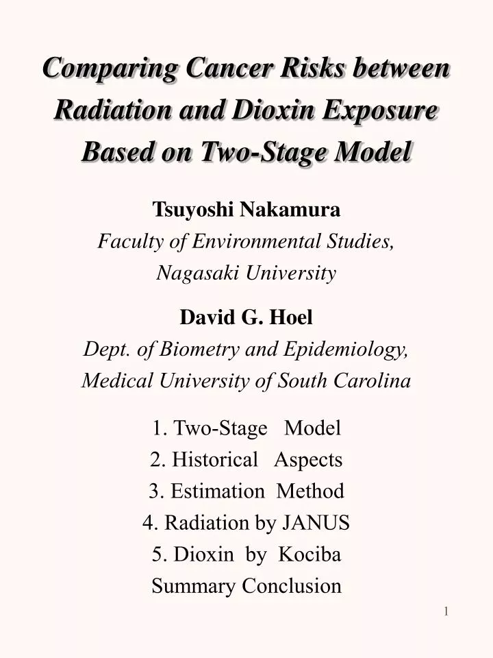
Comparing Cancer Risks between Radiation and Dioxin Exposure Based on Two-Stage Model Tsuyoshi Nakamura Faculty of Environmental Studies, Nagasaki University David G. Hoel Dept. of Biometry and Epidemiology, Medical University of South Carolina 1. Two-Stage Model

E N D
Comparing Cancer Risks between Radiation and Dioxin Exposure Based on Two-Stage Model Tsuyoshi Nakamura Faculty of Environmental Studies, Nagasaki University David G. Hoel Dept. of Biometry and Epidemiology, Medical University of South Carolina 1. Two-Stage Model 2. Historical Aspects 3. Estimation Method 4. Radiation by JANUS 5. Dioxin by Kociba Summary Conclusion
Two-Stage Model Three States of Cells Normal, Intermediate and Malignant N I M Four Parameters for Rates m1 : First Mutation Rate for NI b : Clonal Expansion Rate for I d : Death Rate for I m2 : Second Mutation Rate for IM
History Mathematical tool based on Molecular biology to study Mechanistic processes in Cancer development (Moolgavkar, Venzon, Knudson, 70’s) Special Feature Explicit modeling of Clonal expansion, Differentiation and Mutation of I-cells as a Continuous Stochastic Process Cancer Incidence Data (time, type, covariate) (t, 1, x): endpoint (t, 0, x): censored
Problems Unidentifiability All parameters are not identifiable. Reparameterization or Assumption is necessary. Non-Convergence MLE of the identifiable parameters are still often hardly obtainable, because of the peculiar shape of the likelihood surface (Portier et at. 1997). Non-Standard Algorithm Lack of Confidence in Results Lack of Comparison among Studies
Survivor function S(t) Probability of No Malignant Cell at t, is obtained by solving a series of differential equations, derived from Stochastic processes on Probability Generating Function (Moolgavkar et al 1990; Kopp et al 1994; Portier et al 1996;) Stochastic processes M(t)=(x(t),y(t),z(t)) denote the number of N-, I- and M-cells at t, respectively. M(t): Continuous Markov Birth-Death process S(t)= Si,jProb{M(t)=(i,j,0)}
Probability Generating Function P(i,j,k|t)=Prob{M(t)=(i,j,k) | M(0)=(1,0,0) } G(u,v,w|t)= Si,j,k P(i,j,k|t)uivjwk and Q(i,j,k|t)=Prob{M(t)=(i,j,k) | M(0)=(0,1,0) } H(u,v,w|t)= Si,j,k Q(i,j,k|t)uivjwk S(t)=Si,jP(i,j,0|t)=G(1,1,0|t) Differential Equations It follows that (Portier et al 1996) dG(t)/dt= m1G(t)H(t)-m1G (t) dH(t)/dt= bH(t)2+d-(b+d+m2)H(t) G(0)=1, H(0)=1
Survivor Function S(t) X0 = Number of N-cells, Large and Constant u = NI Rate per Cell per unit Time ==> m1=uX0 S(t)=exp{-L(t)}, L(t)=h{t(R+y)/2+log[{R-y+(R+y)e-Rt}/2R]} L is Cumulative Hazard with new parameters h=m1/b, y=b-d-m2 and R2=(b-d-m2)2+4bm2 Original likelihood y: Net Proliferation Rate r=m1m2=h(R2-y2)/4:Overall Mutation Rate l(h,y,r) based on L(t) is termed Original likelihood. Non-convergence is frequent !
L(t|d=0)= [ ] Conditional likelihood Put d=0 then m*1, b* and m*2 are employedto emphasize these parameters are valid only when d=0 l(m*1,b*,m*2) based on L(t|d=0) is termed Conditional likelihood. Looks Better Shape!
Transformation Conditional likelihood converges better! Biological interpretation of parameters is ? It ignores the death of the I-cells. Biological parameters estimated by m*1, b* and m*2 are h=m*1/b*, y=b*-m*2and r=m*1m*2 (Nakamura and Hoel2002) Thus, MLE of h, y and r are obtained from Conditional Likelihood ! Practically y=b*, since m*2 is small
Comparison on Experimental Data Conditional vs Original JANUS data for Radiation Risk study On g and Neutron in Mice Argonne National Laboratory (1953-1970 ) Reliable Pathological information Kociba data for Chronic Toxicity study on TCDD in Rats Dow Chemical (1978) Reliable Pathological information
Illustration of Two-Stage Model b m2 m1=uX0 d Cited from Moolgavkar(1999) Statitics for the Environment4, Wiley
Control mice 3707 with 1894 Cancer Conditional Likelihood: l =-13692.7, ||U||< 0.001 Parameter Estimate SE log m*1 -4.7618 0.10524 log b*-4.8182 0.03767 log m*2 -12.898 0.13539 logr -17.660 0.1760 logh0.05632 0.1244 Original likelihood: l = -13692.7, ||U||<0.001 Parameter Estimate SE logh 0.05632 0.16436 logy -4.8185 0.04563 logr-17.660 0.2086 Initial Trial Values are assigned as h0=m*1/b*, y0=b* andr0=m*1m*2
Regression Model logq=a+bDose (Contol + g) 7402 mice with 4133 Cancer ConditionalLikelihood: l=-29446.65, ||U||=0.002 Const.a (SE) Slope b (SE) logm*1 -4.931 (0.0817) 0.00717 (0.00115) logb*-4.851 (0.0278)-0.000345 (0.000071) logm*2 -12.43 (0.1014) -0.002934 (0.001126) logr -17.37 (0.1181) 0.00424 (0.000241) -------------------------------------------------------------------------------------------------------------------------------------------------- Original likelihood: l=-29446.69, ||U||=0.2542 Const.a (SE) Slope b (SE) logh-0.0797 (0.1318) 0.00749 (0.00131) logy-4.852 (0.0373)0.000345 (0.000077) logr -17.37 (0.1536) 0.00424 (0.000266) All Estimates are of p<0.01
Effect of Exposure on Mutation and Promotion 1) r=m1m2=uX0m2 2) X0 is Constant not affected by Exposure 3) Effect of exposure on u and that on m2 are the same ( Moolgavkar et al ,1999), 4) logr=a+bDose ==> Dose effect on u and that on m2 is b/2 Dose Effect on Mutation Rate and Net proliferation Rate may be obtained from Conditional likelihood without Additional Assumption!
Log Cumulative Hazards Two-Stage (H) vs K-M(V) Dose 0 :Subjects 3707 Cancer 1894 V H
Log Cumulative Hazards Two-Stage (H) vs K-M(V) Dose 86 : Subjects 1376Cancer 960 V H
Log Cumulative Hazards Two-Stage (H) vs K-M(V) Dose 756 : Subjects 396Cancer 190 V H
Regression Coefficients for Dioxin 205 rats,31 cancer, logq=a+blog(1+Dose) Conditional Likelihood:l= -206.77,||U||=0.0004 Const. SE Slope SE logm*1 -3.780 0.7075non logb*-3.961 0.1062 0.0680 0.01497 logm*2-20.82 1.371 non logr -24.601.259 non Original Likelihood:l= -207.012, ||U||= 0.0012 Const.a SE Slope SE logh0.0865 0.8192non logy-3.979 0.10830.06580.01466 logr -24.32 1.216 non Original Likelihood:l=-207.585, ||U||=5.7489 Incomplete-convergent case Const. SE Slope SE logh-0.47240.7395 non logy-3.773 0.045890.06310.0200 logr -27.140.3368 non
100 10 1 0 Log Cumulative Hazards for Dioxin Doses week
756 400 197.6 86.31 43.15 0 Log Cumulative Hazards for Radiation Doses week