Download
1 / 20
200 likes | 515 Views
Study of the Determinants of Demand for Propane. Prepared and Presented By: Joe Looney J.D. Laing Ernest Sonyi. Background. Propane is used for: Heating homes Heating water Cooking Drying clothes Fueling gas fireplaces As an alternative fuel for vehicles. Background.

E N D
Study of the Determinants of Demand for Propane Prepared and Presented By: Joe Looney J.D. Laing Ernest Sonyi
Background • Propane is used for: • Heating homes • Heating water • Cooking • Drying clothes • Fueling gas fireplaces • As an alternative fuel for vehicles
Background • Propane is used in the Petrochemical industry to make: • Plastics • Alcohols • Fibers • Cosmetics
Background • Propane is used in agriculture for: • Crop drying • Weed control • Fuel for farm equipment • Fuel for irrigation pumps
Objectives • To determine the variables and interactions of these variables upon the demand for propane in the United States • Attempt to use econometric data to show a direct relationship between propane prices and propane demand
Assumptions • The weekly supply data for propane reflects a replenishment of used stores of the product in the market • Meets all five assumptions for regression • The model makes sense • There is a significant statistical relationship between variables • There is an acceptable percent variation between variables • There is no problem with autocorrelation • There is no problem with multicollinearity
Hypotheses • H1: Demand for Propane is explained by poultry production • H2: Demand for Propane is explained temperature • H3: Demand for Propane is explained by prices • H4: Demand for Propane is seasonal
Variables • Dependent Variable • Weekly quantity of Propane supplied to the market • Independent Variables • Weekly poultry slaughter counts • Used as a measure of Agricultural impact on demand • Spot Prices for Propane in Texas, the Midwest and Northwest Europe • Weekly temperature average for the United States • Weekly temperature averages for the Northwest, Northeast, Southwest and Southeast regions of the United States
Endogenous U.S. demand for propane Exogenous Temperature averages Poultry slaughter rates Propane prices Variable Identification
Methodology • Used WinORS to analyze data • Weekly data was collected covering the time span between 2004 and 2007 • Stepwise regression was used to identify the statistically significant variables • Ordinary Least Squares was used to test for: • Normality • Homoscedasticity • Autocorrelation • Multicollinearity
Linear Demand Model Qx = 2226.016 -2.352Tx -7.154Ux-5.108Nx-127.42D1-262.222D2-122.885D3 Qx = Weekly quantity of propane supplied Tx = Weekly spot price of propane in Texas Ux = Weekly temperature average for the US Nx = Weekly temperature average for the Northeast US D1 = Spring Dummy Variable D2 = Summer Dummy Variable D3 = Fall Dummy Variable *all other variables were determined statistically insignificant by the stepwise model
Statistical Significance and Coefficient of Determination • The P-Value is 0.00001 therefore it satisfies the 99% confidence interval Root MSE 154.774 SSQ(Res) 3808838.392 Dep. Mean 1234.163 Coef. Of Var. (CV) 12.541% R-Squared 74.089% Adj R-Squared 73.111%
Homoscedasticity and Normality • P-value for White’s is > .05 therefore the data is homoscedastic • Correlation for Normality is below the approx. Critical Value therefore the data is not normal (flaw of this model) White's Test for Homoscedasticity 6.81 P-value for White’s 0.86988 Correlation for Normality 0.9945 Approx. Critical Value 0.999
Autocorrelation • Durbin value should be > 2, in this case the value is close enough to not reject the data Rho 0.019 Durbin 1.935 Durbin H n/c D Lower Limit 1.651 D Upper Limit 1.817 Ho: Rho = 0 Rho: Pos & Neg Do Not Reject Rho: Positive Do Not Reject Rho: Negative Do Not Reject
Multicollinearity (VIF) • All values for VIF for all independent variables should be less than 10 to ensure no multicollinearity
Elasticity • The elasticity of all the independent variables is inverse and inelastic
Conclusions • We reject the hypotheses that the demand for propane is explained by poultry production or temperature • We accept only the hypotheses that demand for propane is seasonal and is explained by prices specifically the spot price of propane in Mont Belvieu, TX • The only flaw in the model is that the data may not be normal because the correlation for normality is just below the approx. critical value • The spot price of propane in Mont Belvieu, TX is inversely inelastic to the demand for propane in the U.S. with an elasticity of -0.18828, therefore a 10% increase in the spot price would result in only a decrease of 1.8% in demand nationally