Download
1 / 35
350 likes | 480 Views
Lyapunov Functions and Memory. Justin Chumbley. Why do we need more than linear analysis? What is Lyapunov theory? Its components? What does it bring? Application: episodic learning/memory. Linearized stability of non-linear systems: Failures.

E N D
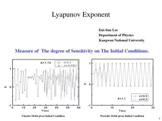
Lyapunov Functions and Memory Justin Chumbley
Why do we need more than linear analysis? • What is Lyapunov theory? • Its components? • What does it bring? • Application: episodic learning/memory
Linearized stability of non-linear systems: Failures • Is there a steady state under pure imaginary eigenvalues? • theorem 8 doesn’t say • Size/Nature of Basin of attractions? • cfa small neighborhood of the ss (linearizing) • Lyapunov • Geometric interpretation of state-space trajectories
Important geometric concepts(in 2d for convenience) • State function • scalar function U of system with continuous partial derivatives • A landscape • Define a landscape with steady state at the bottom of a valley
e.g. • Unique singular point at 0 • Not unique U
* • U defines the valley • Do state trajectories travel downhill? Temporal change of pdstate function along trajectories? • Time implicit in U
e.g. • N-dim case
Lyapunov functions and asymptotic stability • Intuition • Water down a valley all trajectories in a neighborhood approach singular point as
Ch 8 Hopf bifurcation • Van der Pol model for a heart-beat • Analyzed at bifurcation point (where linearized eigenvalues are purely imaginary) • At this point… (0,0) is the only steady state Linearized analysis can’t be applied (pure imaginary eigs) • But: pd state function has time derivates along trajectories
satisfies b • So • Except on x,yaxes where • But when x = 0 then trajectories will move to points where • SoU is a Lyapunov function for … • Ss at (0,0) is asymptotically stable Conclusion: have proven stability where linearization fails
Another failure of Theorem 8 • Points ‘sufficiently close’ to asymptotically stable steady state go there as • But U defines ALL points in the valley in which the sslies! • Intuition: any trajectory starting within the valley flows to ss.
Formally • many steady and basins • Assume we have U for • It delimits a region R within which theorem 12 holds • A constraint U<K defines a subregion within the basin
Key concept: closed contour (or spheroid surface in 3d+) that encloses the ss • As long as this region is within R, T12 guarantees that all points go to steady state • K = highest point on valley walls from which nothing can flow out • is a lower bound on the basin (depends on U too!) e.g. use
Where does U come from? • No general rule. • Another e.g. divisive feedback
Memory • Declarative • Episodic • Semantic • Procedural • …
Episodicmemory (thenlearning) • Computationallevel: one-shotpatternlearning& robust recognition(Generalizationoverinputsanddiscriminate) • Learntogeneralize/discriminateappropriately, givenouruncertainty (statistics) • p(f,x) ? p((x) ? …. e.g. regresion/discriminant • Algorithmiclevel: usestabledynamicequilibria • (x) issteady-stateofsystem m, giveninitialcondition x • not smooth generalization (overinputs) • Dynamics • Implementation levelconstraints • Anatomical: Hippocampal ca3 Network • Physiological: Hebbian
m • 16*16 pyramidal • Completely connected but not self-connected • 1 for feedback inhibition If R is a rate/speed, then acceleration of R is a sigmoidal function of PSP No Self connection … is pre-learnt PSP includes inputs: a subset x of neurons exogenously stimulated What is (x) go? Sigma = semi-saturation time constant
Aim • Understandgeneralization/discrimination • Strategy • Input in thebasin will be ‘recognized’ • i.e. identifiedwiththestoredpattern (asympotically) • Lyapunovtheory assessbasinsofattraction Notation: etc…
For reference Can begeneralizedtohigherorder
s ,
Hebb Rule • Empirical results • Implicate cortical and hippocampal NMDA • 100-200ms window for co-occurance • Presynaptic Glu and Postsynaptic depolarisation by backpropogation from postsynaptic axon (Mg ion removal). Chemical events change synapse
For simplicity… • M = max firing rate • (both pre and post must be firing higher than half maximum) • Synapse changes to fixed k when modified • Irreversible synaptic change • All pairs symmetrically coupled
Learning (matlab) • One stimuli • Multiple stimuli
Pros and limitations of Lyapunov theory • More general stability analysis • Basins of attraction • Elegance and power • No algorithm for getting U • Not unique U: each gives lower bound on basin