Download
1 / 21
210 likes | 216 Views
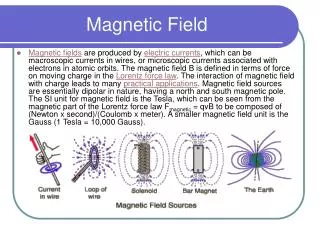
Liquid metal flow under inhomogeneous magnetic field. O. Andreev, E. Votyakov, A. Thess, Y. Kolesnikov. TU Ilmenau, Germany. Electromagnetic Brake (EMBR). magnet system. Main goal. Avoid flow instability. 1. Smooth mean velocity profile. Avoid sources of instability.

E N D
Liquid metal flow under inhomogeneous magnetic field O. Andreev, E. Votyakov,A. Thess, Y. Kolesnikov TU Ilmenau, Germany
ElectromagneticBrake (EMBR) magnet system
Main goal Avoid flow instability 1. Smooth meanvelocity profile Avoid sources of instability 2. Brake generated and introduced velocity fluctuations
N S top view ly side view lx Experimental setup Bz magnetic field Vives probe Plexiglas cover blocks potential probe lx y N In- Ga -Sn S honeycomb inlet contractor permanent magnet outlet diffuser 30 mm
General view of test-section Coordinate system Permanent magnet Channel: S = 210 cm L = 90 cm Liquid metal: GaInSn
B z B max B × F ~ j B ´ - Ñ j = s z V B j / x y z B max 0,5 M-shape velocity profile 0,25 X, mm - 105 - 75 - 45 - 15 15 45 75 105 Y, mm 50 Flow 25 0 0,25 0,5 - 25 B - 50
Governing parameters Reynolds number: Re=U0H/ Re<15000 Hartmann number: Ha=B0H(/)1/2 Ha=400 MHD interaction parameter: N=Ha2/Re N>40 U0 < 35cm/s, B0=0.5T, H=2cm
(a) 3,5 0 3 Flow 2,5 2 x= - 106 mm - 29 20 1 0,5 0 - 0,5 - 50 - 40 - 30 - 20 - 10 0 10 20 30 40 50 Y, mm E y E 0 Streamwise velocity in the middle plane of channel potential velocimetry Re 4000
flow flow Streamwise velocity in the middle plane of channel ultrasound velocimetry Re 4000 magnet
Re =4000 I. turbulence suppression region II. vortical region III. wall jet region % u´/U0 15 12.5 10 7.5 on the axes near walls 5.0 2.5 0 -5 -2.5 0 2.5 5 7.5 10 Decay of velocity fluctuations under the external magnetic field B Magnet Flow
Accuracy ofpotential velocimetryin the region ofinhomogeneousmagnetic fieldis ?!
Principles of potential velocimetry from Ohm’s law y streamwise velocity x physical ERROR of the potential velocimetry measurable values
positivevalues of el.current negative values of el.current positivevalues of el.current directnumericalsimulationbyE. Votyakov,E. Zienike electrical current in the middle plane spanwise Jy electricalcurrent overestimatedvalues of velocity overestimatedvalues of velocity underestimatedvalues
flow flow rate through the channel integral estimation oferror voltmeter potential difference between the side walls movable electrodes onthe side walls
flow 3.5 Re= 3 2716 4014 2.5 overestimatedvalues of flow rate 5312 potentialdifference 6611 2 7909 overestimatedvalues of flow rate 9207 1.5 underestimatedvalues 10505 11804 1 13102 Magnetic field 0.5 flow rate 0 -6 -5 -4 -3 -2 -1 0 1 2 3 4 5 6 x/H, dimensionless streamwise coordinate
Re 4000 flow Comparison of ultrasound and potential velocimetry X/H=0 streamwisevelocity DOP2000 potentialprobe
flow Vivesprobe DOP2000 Comparison of ultrasound and potential velocimetry Re 4000 X/H=-3 streamwisevelocity potentialprobe
flow Vivesprobe DOP2000 Comparison of ultrasound and potential velocimetry Re 4000 X/H=2 streamwisevelocity potentialprobe
flow Vivesprobe DOP2000 potentialprobe Comparison of ultrasound and potential velocimetry Re 4000 X/H=6 streamwisevelocity
flow Vivesprobe DOP2000 Comparison of ultrasound and potential velocimetry Re 4000 X/H=8 streamwisevelocity
Summary remarks • The laboratory flow was investigated in the following range of the governing parameters: Ha = 400, Re<15000, N>10. • Potential probe qualitatively reproduces velocity field within the region of two magnet gaps in streamwise direction. • Vives probe is strongly influenced by the external electric potential and could be applied on the distance which exceeds 5-6 gaps of magnet.