Download
1 / 63
640 likes | 765 Views
Optimal Contracts under Moral Hazard. What does it mean Moral Hazard?. We will use much more often the notion of Moral Hazard as hidden action rather than ex-post hidden information

E N D
What does it mean Moral Hazard? • We will use much more often the notion of Moral Hazard as hidden action rather than ex-post hidden information • Moral Hazard means that the action (effort) that the A supplies after the signature of the contract is not verifiable • This means that the optimal contract cannot be contingent on the effort that the A will exert • Consequently, the optimal contracts will NOT have the form that they used to have when there is SI:: • If e=eopt then principal (P) pays w(xi) to agent (A) if not, then A will pay a lot of money to P
What does the solution to the SI case does not work when there is Moral Hazard? • Say that a Dummy Risk Neutral Principal offers to a Risk Averse A the same contract under moral hazard that he would have offered him if Information is Symmetric • If e=eo then principal (P) paysto agent (A) the fixed wage of: • if not, then A will pay a lot of money to P -Threat is not credible because e is no verifiable -…plus Wage does not change with outcome: no incentives. -RESULT: Agent will exert the lowest possible effort instead of eo
Anticipation to the solution to the optimal contract in case of Moral Hazard • Clearly, if the P wants that the A will exert a given level of effort, she will have to give some incentives • The remuneration schedule will have to change according to outcomes • This implies that the A will have to bear some risk (because the outcome does not only depend on effort but also on luck) • So, the A will have to bear some risk even if the A is risk averse and the P is risk neutral • In case of Moral Hazard, there will not be an efficient allocation of risk
How to compute the optimal contract under MH • For each effort level ei,compute the optimal wi(xi) • Compute P’s expected utility E[B(xi- wi(xi)] for each effort level taking into account the corresponding optimal wi(xi) • Choose the effort and corresponding optimal wi(xi) that gives the largest expected utility for the P • This will be eopt and its corresponding wi(xi) • So, we break the problem into two: • First, compute the optimal wi(xi) for each possible effort • Second, compute the optimal effort (the one that max P’s utility)
Moral Hazard with two possible levels of effort • For simplification, let’s study the situation with only two possible levels of effort: High (eH) and Low (eL) • There are N possible outcomes of the relationship. They follow that: • x1<x2<x3<….<xN • That is, x1 is the worst and xN the best • We label piH the probability of outcome xi when effort is H • We label piL the probability of outcome xi when effort is L
Moral Hazard with two possible levels of effort • For the time being, let’s work in the case in which P is risk neutral and the A is risk averse Now, we should work out the optimal remuneration schedule w(xi) for each level of effort: -Optimal w(xi) for L effort ( this is easy to do) -Optimal w(xi) for H effort ( more difficult)
Optimal w(xi) for low effort • In the case of low effort, we do not need to provide any incentives to the A. • We only need to ensure that the A want to participate (the participation constraint verifies) • Hence, the w(xi) that is optimal under SI is also optimal under MH, that is, a fixed wage equals to: Why is it better this fixed contract that one than a risky one that pays more when the bad outcome is realized?
Optimal w(xi) for High effort • This is much more difficult • We have to solve a new maximization problem…
Optimal w(xi) for High effort • We must solve the following program: The first constraint is the Participation Constraint The second one is called the Incentive compatibility constraint (IIC)
About the IIC • The Incentive Compatibility Constraint tell us that The remuneration scheme w(xi) must be such that the expected utility of exerting high effort will be higher or equal to the expected utility of exerting low effort In this way, the P will be sure that the A will be exerting High Effort, because, given w(xi), it is in the Agent’s own interest to exert high effort
About the IIC • The IIC can be simplified: So:
Optimal w(xi) for High effort • Rewriting the program with the simplified constraints: The first constraint is the Participation Constraint The second one is called the Incentive compatibility constraint (IIC)
Optimal w(xi) for High effort • The Lagrangean would be: Taking the derivative with respect to w(xi), we obtain the first order condition (foc) in page 43 of the book. After manipulating this foc, we obtain equation (3.5) that follows in the next slide…
Optimal w(xi) for High effort Equation (3.5) is: By summing equation (3.5) from i=1 to i=n, we get: This means that in the optimum, the constraint will hold with equality(=) instead of (>=)
Optimal w(xi) for High effort • Notice that (eq 3.5) comes directly from the first order condition, so (eq. 3.5) characterizes the optimal remuneration scheme • Eq. (3.5) can easily be re-arranged as: We know that λ>0. What is the sign of μ? -It cannot be negative, because Lagrange Multipliers cannot be negative in the optimum -Could μ=0?
Optimal w(xi) for High effort If μ was 0, we would have: Intuitively, we know that it cannot be optimal that the Agent is fully insured in this case (see the example of the dummy principal at the beginning of the lecture) So, it cannot be that μ was 0 is zero in the optimum.
Optimal w(xi) for High effort Mathematically: If μ was 0, we would have:
Optimal w(xi) for High effort In summary, if μ was 0 the IC will not be verified !!! We also know that μ cannot be negative in the optimum Necessarily, it must be that μ> 0 This means that the ICC is binding !!! So, in the optimum the constraint will hold with (=), and we can get rid off (>=)
Optimal w(xi) for High effort Now that we know that both constraints (PC, and ICC) are binding, we can use them to find the optimal W(Xi): Notice that these equations might be enough if we only have w(x1) and w(x2). If we have more unknowns, we will also need to use the first order conditions (3.5) or (3.7)
Optimal w(xi) for High effort • The condition that characterizes optimal w(xi) when P is RN and A is RA is (3.5) and equivalently (eq 3.7): -This ratio of probabilities is called the likelihood ratio -So, it is clear that the optimal wage will depend on the outcome of the relationship because different xi will normally imply different values of likelihood ratio and consequently different values of w(xi) ( the wage do change with xi) !!!!
Optimal w(xi) for High effort • The condition that characterizes optimal w(xi) when P is RN and A is RA is (eq 3.7): We can compare this with the result that we obtained under SI (when P is RN and A is RA): So the term in brackets above show up because of Moral Hazard. It was absent when info was symmetric
What does the likelihood ratio: mean? The likelihood ratio indicates the precision with which the result xisignals that the effort level was eH Small likelihood ratio: -piH is large relative to pLi -It is very likely that the effort used was eH when the result xi is observed Example: Clearly, X2 is more informative than X1 about eH was exerted, so it has a smaller likelihood ratio
What is the relation between optimal w(xi) and the likelihood ratio when effort is high? λ >0, we saw it in the previous slides. μ>0, we saw it in the previous slides Notice: small likelihood ratio (signal of eH) implies high w(xi)
An issue of information Assume a RN P that has two shops. A big shop and a small shop. In each shop, the sales can be large or small. For each given of effort, the probability of large sales is the same in each shop The disutility of effort is also the same However, the big shop sells much more than the small shop For the same level of effort, will the optimal remuneration scheme be the same in the large and small shop?
A question of trade-offs… • P is RN and A is RA. This force will tend to minimize risk to the Agent • Effort is no verifiable: This force will tend to make payments to the agent vary according to actual xi (introducing risk), as long as actual xi gives us information about the effort exerted • The optimal remuneration schedule trades off these two forces • Notice that it would not make sense to make the contract contingent on a random variable that: • The agent cannot influence • It is not important for the value of the relationship
When will w(xi) be increasing with xi? If the likelihood ratio is decreasing in i, that is, if higher xi are more informative about eH than lower levels of effort. This is called the monotonous likelihood quotient property. Notice that this property does not necessarily have to hold:
Graphical analysis: P is RN and A is RA. Two outcomes: x1 and x2
Graphical analysis: P is RN and A is RA. Two outcomes: x1 and x2 Draw f(w2,w1) in Fig 3.3, page 59 Now, we need to know how to draw the indifference curves Draw the indifference curves as in Fig 3.3, page 59
Graphical analysis: P is RN and A is RA. Two outcomes: x1 and x2 Their slopes are:
Graphical analysis: P is RN and A is RA. Two outcomes: x1 and x2 x1-w1=x2-w2 For eH x1-w1 For eL x2-w2 Picture of the expected profit lines We can invert the axis, and make Fig 3.4
Graphical analysis: P is RN and A is RA. Two outcomes: x1 and x2 Draw Figures 3.5 and 3.6 -First draw contracts L and H (but call them A & B) -Draw the Indifference curve for low effort through them (in order to measure the utility), and high effort through B -Then say that A will be the optimal contract under SI for eL. -Then say that B is the optimal contract under SI for eH -Explain why A and B are not incentive compatible under MH -Draw the optimal contract under MH: (H’) -Show it is not Pareto Efficient
Optimal Contract with two levels of effort After we have computed the optimal remuneration scheme for High and Low effort, The principal will assess if she prefers High or Low effort levels The optimal contract will be the one that implements her preferred level of effort
Optimal Contract with Moral Hazard • So far, we have studied the case where P is RN and A is RA. If the P wants to implement High Effort, the SI solution (fixed wage) is not incentive compatible, hence a new optimal contract that takes into account the ICC must be computed • Notice that if P is RA and A is RN, then the optimal solution in case of SI (the P will get a fixed rent, and the A will get the outcome minus the rent) is incentive compatible (the A will exert high effort). Consequently: • Moral Hazard does not create problems when the P is RA and the A is RN. The SI solution can be implemented
Just to remind you… Given the differentiable function F(x). If the point x0 is its maximum, then it must be the case that the first derivative of F(x) evaluated at x0 is equal to zero. That is F’(x0)=0 However, other points that are not a maximum, can also satisfy the condition that the first derivative evaluated at them is zero (do a graph…)
Problem with continuous effort.Optimal contract to implement e0 The (IIC) is the last one. It tell us that e0 should maximize the agent’s expected utility given w(xi), so that it is in the Agent’s own interest to carry out e0
Problem with continuous effort.Optimal contract to implement e0 The problem is very difficult to solve as it is because it is a maximization problem within another maximization problem. To simplify it: -If e0 maximizes the agent’s expected utility, it must be the case that the derivative of the agent’s expected utility with respect to effort, evaluated at e0 is zero, that is: Is this restriction equivalent to the ICC of the previous slide? No always… draw a concave and a non-concave function… In a non-concave function, the effort levels that satisfy this second restriction are more than the ones that satisfy the ICC
Problem with continuous effort.Optimal contract to implement e0 Substituting the real ICC by the simplified constraint is called the First Order Approach. When this approach is correct, economists says that the conditions for the first order approach verifies If the expected utility function is concave, then the First Order Approach is valid
Problem with continuous effort.Optimal contract to implement e0Using First Order Approach:
Problem with continuous effort.Optimal contract to implement e0Using First Order Approach:
Problem with continuous effort.Optimal contract to implement e0Using First Order Approach: Notice that w(xi) will depend on the result (sales) because the ratio of the right hand side depends on the results. So, the agent is not fully insured
Problem with continuous effort.Optimal contract to implement e0Using First Order Approach: The previous analysis has given us the optimal remuneration scheme for a given level of effort (e0) Now, we would have to study the optimal level of effort but we will not do that because it is too complicated from a mathematical point of view.
Other issues in optimal contracts under Moral Hazard Limited liability Value of information Contracts based on severe punishments What happens when it is the agent who offers the contract?
Limited liability • Contracts where a P is RN and A is RA under SI followed the following scheme: • If the agent exerts effort e0, he will get the fixed wage w0 if he exerts another effort, he will have to pay to the principal a large sum of money • This contract incorporates a threat to penalize the agent. This threat ensures that the agent does not find attractive to exert a level of effort that is not desired by the principal. • Sometimes, the penalization is not legal or is not credible: • An employee cannot pay to the firm. The firm has always to obey the minimum wage • A bank cannot make the shareholders of a company to pay the company debts if the company goes bankrupt
Limited liability • If the penalization is not legal or it is not credible, the agent can exert a low level of effort even if: • Information is symmetric (no MH) • P is requesting a high level of effort • So, the P will have to use the Incentive Compatibility constraint even if information is symmetric • So, when there is limited liability, the optimal contract might give incentives to the agent even if the P is RN and information is symmetric
The value of information under MH • So far, we have studied that the contract will be contingent only on the result of the relationship (sales). This has been done for simplicity. • Clearly, the principal is interested in using in the contracts signals that reveal new information on the agent’s effort • These signals could be: • Other’s agents results • Control activities • State of Nature (let’s see an example with this)
Example with state of nature.. In this case, it might be very costly to provide incentives so that the agent exerts high effort. This is because even if the agent exerts high effort, the probability of low sales is quite high. This might be because the probability of raining is too high…