Download
1 / 40
410 likes | 759 Views
Representing uncertain knowledge. Points Symbolic and numerical uncertainty The Closed World Assumption Predicate completion Taxonomic hierarchies Abduction Truth maintenance Bayes’s rule Certainty factors Fuzzy sets. Symbolic and numerical uncertainty.

E N D
Representing uncertain knowledge • Points • Symbolic and numerical uncertainty • The Closed World Assumption • Predicate completion • Taxonomic hierarchies • Abduction • Truth maintenance • Bayes’s rule • Certainty factors • Fuzzy sets
Symbolic and numerical uncertainty • Symbolic uncertainty: defeasible reasoning. • Non-monotonic logic:make conclusions that cause no inconsistency. • Default logic. • Modal logic -- necessity and possibility:necessarily Φ ≡ ¬ possibly ¬ Φpossibly Φ ≡ ¬ necessarily ¬ Φ • Numeric uncertainty: statistical reasoning, certainty factors. • Bayesian probability theory. • Fuzzy logic (theory of fuzzy sets).
Examples of approximate reasoning in real life • Judging by general shape, not by details. • Jumping to conclusions without sufficient evidence.(Consider a lawn sign, seen from afar.) • Understanding language. • ... • ...
Why we need more than first-order logic • Complete ↔ incomplete knowledge: • the world cannot be represented completely,there are exceptions and qualified statements. • Generality ↔ specificity (and typicality): • absolute statements ignore individual variety. • Consistency ↔ inconsistency: • conflicting views cannot be represented in first-order logic,not within one theory. • Monotonic ↔ defeasible reasoning: • a change of mind cannot be represented. • Absolute ↔ tentative statements: • partial commitment cannot be represented,statistical tendencies cannot be expressed. • Finality ↔ openness of knowledge: • learning should not only mean new theorems.
The Closed-World Assumption • A complete theory in first-order logic must include either a fact or its negation. • The Closed World Assumption (CWA) states that the only true facts are those that are explicitly listed as true (in a knowledge base, in a database) or are provably true. • We may extend the theory by adding to it explicit negations of facts that cannot be proven. • In Prolog, this principle is implemented by "finite failure", or "negation as failure".
Predicate completion • The factp(a)could be rewritten equivalently as • ∀x x = a p(x) • A completion of this quantified formula is a formula in which we enumerate all objects with property p. In this tiny example: • ∀x p(x) x = a • A larger example: the world of birds. • ∀x ostrich(x) bird(x) • ¬ostrich(Sam) • bird(Tweety) • To complete the predicate bird, we say: • ∀x bird(x)(ostrich(x)x = Tweety) • This allows us to prove, for example, that • ¬bird(Sam)
Predicate completion (2) • How to achieve non-monotonic reasoning? Let us add a new formula: • ∀x penguin(x) bird(x) • ∀x ostrich(x) bird(x) • ¬ostrich(Sam) • bird(Tweety) • A new completion of the predicate bird would be: • ∀x bird(x) • (ostrich(x) penguin(x) x = Tweety) • We cannot prove ¬bird(Sam) any more (why?).
Taxonomic hierarchies and defaults • thing(Tweety) • bird(x) thing(x) • ostrich(x) bird(x) • flying-ostrich(x) ostrich(x) • The following set of formulae represents typicality and exceptions: • thing(x) ¬bird(x) ¬flies(x) • bird(x) ¬ostrich(x) flies(x) • ostrich(x) ¬flying-ostrich(x) • ¬flies(x) • flying-ostrich(x) flies(x)
Taxonomic hierarchies and defaults (2) • This works, but is too specific. We need a way of showing exceptions explicitly. An exception is a departure from normality, and a way of blocking inheritance: • thing(x) ¬abnormalt(x) ¬flies(x) • bird(x) abnormalt(x) • bird(x) ¬abnormalb(x) flies(x) • ostrich(x) abnormalb(x) • ostrich(x) ¬abnormalo(x) ¬flies(x) • flying-ostrich(x) abnormalo(x) • flying-ostrich(x) flies(x)
Taxonomic hierarchies and defaults (3) • The taxonomy is now as follows: • flying-ostrich(x) ostrich(x) • flying-ostrich(x) abnormalo(x) • ostrich(x) bird(x) • ostrich(x) abnormalb(x) • bird(x) thing(x) • bird(x) abnormalt(x) • thing(Tweety) • The properties of classes: • thing(x) ¬abnormalt(x) ¬flies(x) • bird(x) ¬abnormalb(x) flies(x) • ostrich(x) ¬abnormalo(x) ¬flies(x) • flying-ostrich(x) flies(x)
Taxonomic hierarchies and defaults (4) • This kind of formulae can be used to deduce properties of objects, if we can also supply the completion. For example, does Tweety fly? • The completion: • thing(x) bird(x) x = Tweety • bird(x) ostrich(x) • ostrich(x) flying-ostrich(x) • abnormalt(x) bird(x) • abnormalb(x) ostrich(x) • abnormalo(x) flying-ostrich(x) • ¬flying-ostrich(x)
Taxonomic hierarchies and defaults (5) • The last formula is equivalent to • flying-ostrich(x) false • which reflects the fact that no taxonomical rule has flying-ostrich as a conclusion. • We can now prove all of these: • ¬flying-ostrich(Tweety) • ¬ostrich(Tweety) • ¬bird(Tweety) • ¬abnormalt(Tweety) • so we can show that • ¬flies(Tweety)
Taxonomic hierarchies and defaults (6) • This hierarchy again can be changed non-monotonically. Suppose that we add • bird(Tweety) • to the taxonomy. • The new completion of the predicate bird will be: • bird(x) ostrich(x) x = Tweety • instead of • bird(x) ostrich(x) • We will not be able to prove • ¬abnormalt(Tweety) • any more. We will, however, be able to prove • ¬abnormalb(Tweety)
A quaker and a republican • Quakers are pacifists. Republicans are not pacifists. Richard is a republican and a quaker. Is he a pacifist? • These rules are ambiguous. Let us clarify: • Only a typical quaker is a pacifist. Only a typical republican is not a pacifist. • This can be expressed in terms of consistency: • ∀x quaker(x) CONSISTENT(pacifist(x)) pacifist(x) • ∀x republican(x) CONSISTENT(¬pacifist(x)) ¬pacifist(x) • If we apply the first rule to Richard, we find he is a pacifist (nothing contradicts this conclusion), but then the second rule cannot be used—and vice versa. In effect, neither pacifist(x) nor ¬pacifist(x) can be proven.
Abduction ... demonstrated on one example • Abduction means systematic guessing: "infer" an assumption from a conclusion. For example, the following formula: • ∀x rainedOn(x) wet(x) • could be used "backwards" with a specific x: • ifwet(Tree)thenrainedOn(Tree) • This, however, would not be logically justified. We could say: • wet(Tree) CONSISTENT(rainedOn(Tree)) rainedOn(Tree) • We could also attach probabilities, for example like this: • wet(Tree) rainedOn(Tree) || 70% • wet(Tree) morningDewOn(Tree) || 20% • wet(Tree) sprinkled(Tree) || 10%
happy(a) truth value: UNKNOWN justification: none happy(b) truth value: UNKNOWN justification: none happy (a) happy(b) truth value: TRUE justification: given Truth maintenance The first formula arrives:we build a partial network. happy(a) happy(b) • … demonstrated on one example
happy(a) truth value: TRUE justification: given happy(b) truth value: TRUE justification: deduced happy (a) happy(b) truth value: TRUE justification: given Truth maintenance (2) A new fact: incorporate itinto the network. happy(a)
happy(a) truth value: TRUE justification: given happy (a) happy(b) truth value: TRUE justification: given happy (b) happy(c) truth value: TRUE justification: given happy(b) truth value: TRUE justification: deduced happy(c) truth value: TRUE justification: deduced happy(d) truth value: TRUE justification: given Truth maintenance (3) A new rule and a new fact: happy(b) happy(c) happy(d)
happy(a) truth value: TRUE justification: given happy (a) happy(b) truth value: TRUE justification: given happy(b) truth value: TRUE justification: deduced happy (b) happy(c) truth value: TRUE justification: given happy(c) truth value: TRUE justification: deduced happy (d) happy(c) truth value: TRUE justification: given happy(c) truth value: TRUE justification: deduced happy(d) truth value: TRUE justification: given Truth maintenance (4) This rule causes trouble: happy(d) happy(c)
happy(a) truth value: TRUE justification: given happy (a) happy(b) truth value: TRUE justification: given happy(b) truth value: TRUE justification: deduced happy (b) happy(c) truth value: TRUE justification: given happy(c) truth value: TRUE justification: deduced happy (d) happy(c) truth value: FALSE justification:assumed happy(d) truth value: TRUE justification: given Truth maintenance (5) One possible fix: disable happy(d) happy(c)
happy(a) truth value: TRUE justification: given happy (a) happy(b) truth value: TRUE justification: given happy(b) truth value: TRUE justification: deduced happy (b) happy(c) truth value: FALSE justification:assumed happy (d) happy(c) truth value: TRUE justification: given happy(c) truth value: TRUE justification: deduced happy(d) truth value: TRUE justification: given Truth maintenance (6) Another fix: disable happy(b) happy(c)
Bayes’s theorem • Bayesian probability theory. • Fuzzy logic (only signalled here). • Dempster-Shafer theory (not discussed here). • Bayes's theorem allows us to compute how probable it is that a hypothesis Hi follows from a piece of evidence E (for example, from a symptom or a measurement). • The required data: the probability of Hj and the probability of E given Hj for all possible hypotheses.
Bayes’s theorem (2) • Medical diagnosis is a handy example. A patient may have a cold, a flu, pneumonia, rheumatism, and so on. The usual symptoms are high fever, short breath, runny nose, and so on. • We need the probabilities (based on statistical data?) of all diseases, and the probabilities of high fever, short breath, runny nose in the case of a cold, a flu, pneumonia, rheumatism. [This is asking a lot!] • We would also like to assume that all relationships between Hj and E are mutually independent. [This is asking even more!]
p( E | Hi ) * p( Hi ) p( Hi | E ) = ————————— p( E | Hj ) * p( Hj ) j Bayes’s theorem (3) • The probability data: • p( Hi | E ) the probability of Hi given E. • p( Hi ) the overall probability of Hi. • p( E | Hi ) the probability of observing E given Hi. • Bayes' theorem
p( E | Hi ) * p( Hi ) p( Hi | E ) = ————————— p( E ) Bayes’s theorem (4) • If we assume that all the conditional probabilities under summation are independent, we can simplify the formula:
Bayes’s theorem (5) Example • "A poker player closes one eye 9 times out of 10 before passing a hand. He passes 50% of the hands, and closes one eye during 60% of the hands. What is the probability that he will pass a hand given that he closes one eye?" • Hj: the player passes a hand. • E: the player closes one eye. • p( E | Hj ) = 0.9 • p( E ) = 0.6 • p( Hj ) = 0.5 • p( Hj | E ) = 0.9 * 0.5 / 0.6 = 0.75
p( E | H ) * p( H ) p( H | E ) = ————————— p( E ) p( E | H ) * p( H ) p( H | E ) = ————————— p( E ) Odds calculation • Yet another version of Bayes’s formula is based on the concepts of odds and likelihood.
p( E | H ) * p( H ) p( H | E ) ————— = ————————— p( H | E ) p( E | H ) * p( H ) p( e ) p( e ) O( e ) = ———— = ————— 1 - p( e ) p( e ) Odds calculation (2) • These two formulae give this: The odds of event e: We note that p( H | E ) + p( ¬H | E) = 1.
p( E | H ) O( H | E ) = —————— * O( H ) p( E | H ) Odds calculation (3) Define the fraction as the likelihood ratio (E, H) of a piece of evidence E with respect to hypothesis H: O( H | E ) = (E, H) * O( H ) An intuition: how to compute the new odds of H (given additional evidence E) from the previous odds of H. > 1 strengthens our belief in H.
Odds calculation (4) Example 25% of students in the AI course get an A. 80% of students who get an A do all homework. 60% of students who do not get an A do all homework. 75% of students who get an A are CS majors. 50% of students who do not get an A are CS majors. Irene does all her homework is the AI course. Mary is a CS major and does all her homework. What are Irene's and Mary's odds of getting an A? Let A = "gets an A". C = "is a CS major". W = "does all homework".
p( W | A ) * p( A ) p( A | W ) O( A | W ) = —————— = —————————— p( A | W ) p( W | A ) * p( A ) 0.8 * 0.25 4 = ————— = — 0.6 * 0.75 9 Odds calculation (5) Example p(A) = 0.25 p(W | A) = 0.8 p(W | ¬A) = 0.6 p(C | A) = 0.75 p(C | ¬A) = 0.5
p( CW | A ) * p( A ) p( A | CW ) O( A | CW ) = ——————— = ——————————— p( A | CW ) p( CW | A ) * p( A ) p( C | A ) * p( W | A ) * p( A ) 0.75 * 4 2 = ——————————————— = ———— = — 0.5 * 9 3 p( C | A ) * p( W | A ) * p( A ) Odds calculation (6) Example p(A) = 0.25 p(W | A) = 0.8 p(W | ¬A) = 0.6 p(C | A) = 0.75 p(C | ¬A) = 0.5
The Stanford certainty factor algebra Textbook, section 9.2.1 • MB(H | E): the measure of belief in H given E. • MD(H | E): the measure of disbelief in H given E. • Each piece of evidence must be either for or against a hypothesis: • either 0 < MB(H | E) < 1 while MD(H | E) = 0, • or 0 < MD(H | E) < 1 while MB(H | E) = 0. • The certainty factor is: • CF(H | E) = MB(H | E) - MD(H | E)
The Stanford certainty factor algebra (2) • Certainty factors are attached to premises of rules in production systems (it started with MYCIN). We need to calculate the CF for conjunctions and disjunctions: • CF(P1 P2) = min( CF(P1), CF(P2) ) • CF(P1 P2) = max( CF(P1), CF(P2) ) • We also need to compute the CF of a result supported by two rules with factors CF1 and CF2: • CF1 + CF2 - CF1 * CF2 when CF1 > 0, CF2 > 0, • CF1 + CF2 + CF1* CF2 when CF1 < 0, CF2 < 0, CF1 + CF2 ————————— when signs differ. 1 - min(|CF1|, |CF2|)
{ 0 if sC C(s) = 1 if sC { 0.0 if sis not inF F(s) = 0.0 < m < 1.0 if sis partially inF 1.0 if sis totally inF Read: textbook, section 9.2.2 Fuzzy sets A crisp set CSis defined by a characteristic functionC(s): S {0, 1}. A fuzzy set FSis defined by a membership functionF(s): S [0.0, 1.0]. F(s) describes to what degrees belongs to F: 1.0 means "definitely belongs", 0.0 means "definitely does not belong", other values indicate intermediate "degrees” of belonging.
Fuzzy sets (2) Range of logical values in Boolean and fuzzy logic ©Negnevitsky 2002
Fuzzy sets (3) • Consider N, the set of positive integers. • Let FN be the set of "small integers”. • Let F be like this: • F(1) = 1.0 • F(2) = 1.0 • F(3) = 0.9 • F(4) = 0.8 • ... • F(50) = 0.001 • ... • F defines a probability distribution for statements such as "X is a small integer".
Fuzzy sets (4) Tall men ©Negnevitsky 2002
Fuzzy sets (5) Sets of short, average and tall men .. and a man 184 cm tall ©Negnevitsky 2002
Fuzzy sets (6) Basic operations on fuzzy sets A(x) = 1 - A(x) A B(x) = min (A(x), B(x)) = A(x) B(x) A B(x) = max (A(x), B(x)) = A(x) B(x) This is the tip of a (fuzzy) iceberg. We have fuzzy “logic” and fuzzy rules, fuzzy inference, fuzzy expert systems, and so on. Even fuzzy cubes... http://ceeserver.cee.cornell.edu/asce/ConcreteCanoe/Icebreaker/pics/nonraceday/fuzzy_cubes.JPG