Download
1 / 1
10 likes | 165 Views
6 Dynamic programming In the preceding chapters we have seen some elegant design principles.such as divide- andconquer , graph exploration, and greedy choice.that yield denitive algorithms for a variety

E N D
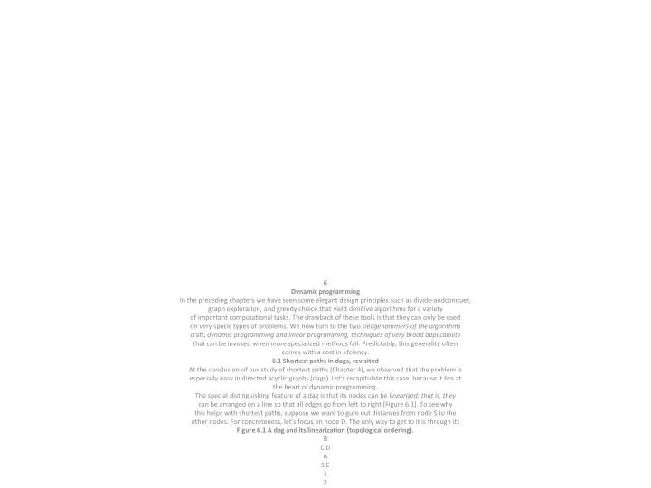
6 Dynamic programming In the preceding chapters we have seen some elegant design principles.such as divide-andconquer, graph exploration, and greedy choice.that yield denitive algorithms for a variety of important computational tasks. The drawback of these tools is that they can only be used on very specic types of problems. We now turn to the two sledgehammers of the algorithms craft, dynamic programming and linear programming, techniques of very broad applicability that can be invoked when more specialized methods fail. Predictably, this generality often comes with a cost in efciency. 6.1 Shortest paths in dags, revisited At the conclusion of our study of shortest paths (Chapter 4), we observed that the problem is especially easy in directed acyclic graphs (dags). Let's recapitulate this case, because it lies at the heart of dynamic programming. The special distinguishing feature of a dag is that its nodes can be linearized; that is, they can be arranged on a line so that all edges go from left to right (Figure 6.1). To see why this helps with shortest paths, suppose we want to gure out distances from node S to the other nodes. For concreteness, let's focus on node D. The only way to get to it is through its Figure 6.1 A dag and its linearization (topological ordering). B C D A S E 1 2 4 1 6 3 1 2 S C 4 A 6 B D E 3 1 2 1 1 2 169 170 Algorithms predecessors, B or C; so to nd the shortest path to D, we need only compare these two routes: dist(D) = minfdist(B) + 1; dist(C) + 3g: A similar relation can be written for every node. If we compute these dist values in the left-to-right order of Figure 6.1, we can always be sure that by the time we get to a node v, we already have all the information we need to compute dist(v). We are therefore able to compute all distances in a single pass: initialize all dist() values to 1 dist(s) = 0 for each v 2 V nfsg, in linearized order: dist(v) = min(u;v)2Efdist(u) + l(u; v)g Notice that this algorithm is solving a collection of subproblems, fdist(u) : u 2 V g. We start with the smallest of them, dist(s), since we immediately know its answer to be 0. We then proceed with progressively .larger. subproblems.distances to vertices that are further and further along in the linearization.where we are thinking of a subproblem as large if we need to have solved a lot of other subproblems before we can get to it. This is a very general technique. At each node, we compute some function of the values of the node's predecessors. It so happens that our particular function is a minimum of sums, but we could just as well make it a maximum, in which case we would get longest paths in the dag. Or we could use a product instead of a sum inside the brackets, in which case we would end up computing the path with the smallest product of edge lengths. Dynamic programming is a very powerful algorithmic paradigm in which a problem is solved by identifying a collection of subproblems and tackling them one by one, smallest rst, using the answers to small problems to help gure out larger ones, until the whole lot of them is solved. In dynamic programming we are not given a dag; the dag is implicit. Its nodes are the subproblems we dene, and its edges are the dependencies between the subproblems: if to solve subproblem B we need the answer to subproblem A, then there is a (conceptual) edge from A to B. In this case, A is thought of as a smaller subproblem than B.and it will always be smaller, in an obvious sense. But it's time we saw an example. 6.2 Longest increasing subsequences In the longest increasing subsequence problem, the input is a sequence of numbers a1; : : : ; an. A subsequence is any subset of these numbers taken in order, of the form ai1 ; ai2 ; : : : ; aik where 1 i1 < i2 < < ik n, and an increasing subsequence is one in which the numbers are getting strictly larger. The task is to nd the increasing subsequence of greatest length. For instance, the longest increasing subsequence of 5; 2; 8; 6; 3; 6; 9; 7 is 2; 3; 6; 9: 5 2 8 6 3 6 9 7 S. Dasgupta, C.H. Papadimitriou, and U.V. Vazirani 171 Figure 6.2 The dag of increasing subsequences. 5 2 8 6 3 6 9 7 In this example, the arrows denote transitions between consecutive elements of the optimal solution. More generally, to better understand the solution space, let's create a graph of all permissible transitions: establish a node i for each element ai, and add directed edges (i; j) whenever it is possible for ai and aj to be consecutive elements in an increasing subsequence, that is, whenever i < j and ai < aj (Figure 6.2). Notice that (1) this graph G = (V;E) is a dag, since all edges (i; j) have i < j, and (2) there is a one-to-one correspondence between increasing subsequences and paths in this dag. Therefore, our goal is simply to nd the longest path in the dag! Here is the algorithm: for j = 1; 2; : : : ; n: L(j) = 1 + maxfL(i) : (i; j) 2 Eg return maxj L(j) L(j) is the length of the longest path.the longest increasing subsequence.ending at j (plus 1, since strictly speaking we need to count nodes on the path, not edges). By reasoning in the same way as we did for shortest paths, we see that any path to node j must pass through one of its predecessors, and therefore L(j) is 1 plus the maximum L() value of these predecessors. If there are no edges into j, we take the maximum over the empty set, zero. And the nal answer is the largest L(j), since any ending position is allowed. This is dynamic programming. In order to solve our original problem, we have dened a collection of subproblemsfL(j) : 1 j ng with the following key property that allows them to be solved in a single pass: (*) There is an ordering on the subproblems, and a relation that shows how to solve a subproblem given the answers to .smaller. subproblems, that is, subproblems that appear earlier in the ordering. In our case, each subproblem is solved using the relation L(j) = 1 + maxfL(i) : (i; j) 2 Eg; 172 Algorithms an expression which involves only smaller subproblems. How long does this step take? It requires the predecessors of j to be known; for this the adjacency list of the reverse graph GR, constructible in linear time (recall Exercise 3.5), is handy. The computation of L(j) then takes time proportional to the indegree of j, giving an overall running time linear in jEj. This is at most O(n2), the maximum being when the input array is sorted in increasing order. Thus the dynamic programming solution is both simple and efcient. There is one last issue to be cleared up: the L-values only tell us the length of the optimal subsequence, so how do we recover the subsequence itself? This is easily managed with the same bookkeeping device we used for shortest paths in Chapter 4. While computing L(j), we should also note down prev(j), the next-to-last node on the longest path to j. The optimal subsequence can then be reconstructed by following these backpointers.