Download
1 / 35
350 likes | 445 Views
This course, offered by the University of Iowa's Department of Mathematics, focuses on the applications of algebraic topology, particularly cohomology, in scientific and engineering fields. Designed for continuing education, the curriculum includes practical approaches such as Zigzag Persistence for topological data analysis and dimensionality reduction techniques. Participants will explore tools and concepts essential for analyzing complex data structures, including gene expression datasets and more, through Python programming.

E N D
MATH:7450 (22M:305) Topics in Topology: Scientific and Engineering Applications of Algebraic Topology Oct 21, 2013: Cohomology Fall 2013 course offered through the University of Iowa Division of Continuing Education Isabel K. Darcy, Department of Mathematics Applied Mathematical and Computational Sciences, University of Iowa http://www.math.uiowa.edu/~idarcy/AppliedTopology.html
triangle-zigzag.py from dionysus import Simplex, ZigzagPersistence, \ vertex_cmp, data_cmp \ # ,enable_log complex = {Simplex((0,), 0): None, # A Simplex((1,), 1): None, # B Simplex((2,), 2): None, # C Simplex((0,1), 2.5): None, # AB Simplex((1,2), 2.9): None, # BC Simplex((0,2), 3.5): None, # CA Simplex((0,1,2), 5): None} # ABC
print "Complex:" for s in sorted(complex.keys()): print s print triangle idarcy$ python2.7 triangle-zigzag.py Complex: <0> <1> <2> <0, 1> 2.500000 <1, 2> 2.900000 <0, 2> 3.500000 <0, 1, 2>
#enable_log("topology/persistence") zz = ZigzagPersistence() # Add all the simplices b = 1 for s in sorted(complex.keys(), data_cmp): print "%d: Adding %s" % (b, s) 1: Adding <0> 2: Adding <1> 3: Adding <2> 0 1 2
# Add all the simplices b = 1 for s in sorted(complex.keys(), data_cmp): print "%d: Adding %s" % (b, s) i,d = zz.add([complex[ss] for ss in s.boundary], b) complex[s] = i if d: print "Interval (%d, %d)" % (d, b-1) b += 1
# Add all the simplices b = 1 for s in sorted(complex.keys(), data_cmp): print "%d: Adding %s" % (b, s) i,d = zz.add([complex[ss] for ss in s.boundary], b) complex[s] = i if d: print "Interval (%d, %d)" % (d, b-1) b += 1 4: Adding <0, 1> 2.500000 Interval (2, 3) 5: Adding <1, 2> 2.900000 Interval (3, 4) 6: Adding <0, 2> 3.500000 7: Adding <0, 1, 2> Interval (6, 6) 0 1 2
# Remove all the simplices for s in sorted(complex.keys(), data_cmp, reverse = True): print "%d: Removing %s" % (b, s) d = zz.remove(complex[s], b) del complex[s] if d: print "Interval (%d, %d)" % (d, b-1) b += 1 8: Removing <0, 1, 2> 9: Removing <0, 2> 3.500000 Interval (8, 8) 10: Removing <1, 2> 2.900000 11: Removing <0, 1> 2.500000 0 1 2
12: Removing <2> Interval (10, 11) 13: Removing <1> Interval (11, 12) 14: Removing <0> Interval (1, 13) 0 1 2
http://link.springer.com/article/10.1007%2Fs00454-011-9344-x
NKI (2002) breast cancer data: • gene expression levels of 24,000 from 272 tumors • Data = 272 points living in R24000
NKI (2002) breast cancer data: • gene expression levels of 24,000 from 272 tumors • Data = 272 points living in R24000 • In reality one cleans the data first, removing unreliable data, etc. • One may also remove dimensions (genes) that appear irrelevant.
NKI (2002) breast cancer data: • gene expression levels of 24,000 from 272 tumors • Data = 272 points living in R24000 • Since our dataset consists of only 272 points, it can’t be 24000-dimensional.
For example, suppose our very fake data is { (9, 8, 7, 6, 5, 4, 3, 2, 3) ti | i = 1, 2, 3, … 1000 } = { (9, 8, 7, 6, 5, 4, 3, 2, 3), { (18, 16, 14, 12, 10, 8, 6, 4, 6), … }
Dimensionality Reduction: • Given dataset D RN • Want: embedding f: D Rn where n << N • which “preserves” the structure of the data. • Example: • { (9, 8, 7, 6, 5, 4, 3, 2, 3) ti | i = 1, 2, 3, … 1000 } R9 • f: D R, f((9, 8, 7, 6, 5, 4, 3, 2, 3) ti) = ti U U
Example: Principle component analysis (PCA) http://en.wikipedia.org/wiki/File:GaussianScatterPCA.png
Many reduction methods: f1: D R,f2: D R, …fn: D R (f1, f2, … fn): D Rn Many are linear, M: RN Rn, Mx = y But there are also non-linear dimensionality reduction algorithms.
f1: D R,f2: D R, …fn: D R (f1, f2, … fn): D Rn
Goal f1: D S1,f2: D S1, …fn: D S1
Cohomology and circular coordinates: Let X = finite simplicial complex. X0 = set of 0-simplices = vertices. X1 = set of 1-simplices = edges. X2 = set of 2-simplices = faces. . . . v2 e1 e2 v1 v3 e3
Homology Let X = finite simplicial complex. C0 = set of 0-chains = linear combinations of vertices C1 = set of 1-chains = linear combinations of edges. C2 = set of 2-chains = linear combinations of faces. . . . v2 e1 e2 v1 v3 e3
Cohomology and circular coordinates: Let X = finite simplicial complex, R a ring. C0 = set of 0-cochains = { f : C0 R | f homomorphism} C1 = set of 1-cochains = { f : C1 R | f homomorphism} C2 = set of 2-cochains = { f : C2 R | f homomorphism} . . .
Cohomology and circular coordinates: Let X = finite simplicial complex, R a ring. C0(X, R) = set of 0-cochains = { f : X0 R } C1(X, R) = set of 1-cochains = { f : X1 R } C2(X, R) = set of 2-cochains = { f : X2 R } . . .
Proposition 1: Let α ∈ C1(X;Z) be a cocycle. Then there exists a continuous function θ : X → S1 which maps each vertex to 0, and each edge ab around the entire circle with winding number α(ab). v2 → e1 e2 v1 v3 e3
Proposition 2: 2 Let α ∈ C1(X;R) be a cocycle. Suppose there existsα ∈ C1(X;Z) and f ∈ C0(X;R) such that α = α + d0f . Then there exists a continuous function θ : X → S1 which maps each edge ablinearly to an interval of length α(ab), measured with sign. v2 → e1 e2 v1 v3 e3
coboundarymaps d0: C0 = { f : X0 R } → C1 = { f : X1 R } (d0f )(ab) = f (b)− f (a) d1: C1 = { f : X1 R } → C2= { f : X2 R } (d1α)(abc) = α(bc)− α(ac)+α(ab).
Let α ∈ Ci , di: Ci= { f : Xi R } → Ci+1= { f : Xi+1 R } α is a cocycle if diα = 0. α is a coboundary if there exists f in Ci-1 s.t. di-1f = α Note d1d0 f = 0 for any f ∈ C0. (d0f )(ab) = f (b) − f (a) (d1d0f )(abc) = d0f(bc)− d0f(ac)+ d0f(ab) = d0f(c) - d0f(b)-d0f(c) + d0f(a)+ d0f(b) - d0f(a)
d1 d0 f = 0 implies Im (d0 ) ⊆ Ker (d1 ). H1 (X;A ) = Ker (d1 )/ Im (d0 ). Twococycles α,β arecohomologousif α − β is a coboundary.
d1 d0 f = 0 implies Im (d0 ) ⊆ Ker (d1 ). H1 (X;A ) = Ker (d1 )/ Im (d0 ). v2 e1 e2 v1 v3 e3
d1 d0 f = 0 implies Im (d0 ) ⊆ Ker (d1 ). H1 (X;A ) = Ker (d1 )/ Im (d0 ). v2 0 C0 C1 0 e1 e2 v1 v3 e3
C0(X, R) = set of 0-cochains = { f : X0 R } v2 e1 e2 v1 v3 e3
C0(X, R) = set of 0-cochains = { f : X0 R } = { f | f(v1) = r1, f(v2) = r2, f(v3) = r3; (r1, r2, r3) in R3 } C1(X, R) = set of 1-cochains = { f : X1 R } = { f | f(e1) = r1, f(e2) = r2, f(e3) = r3; (r1, r2, r3) in R3 } v2 e1 e2 v1 v3 e3
C0(X, R) = set of 0-cochains = { f : X0 R } = { f | f(v1) = r1, f(v2) = r2, f(v3) = r3; (r1, r2, r3) in R3 } C1(X, R) = set of 1-cochains = { f : X1 R } = { f | f(e1) = r1, f(e2) = r2, f(e3) = r3; (r1, r2, r3) in R3 } Hi(X;A ) = Ker (di)/ Im (di-1). 0 C0 C1 0 v2 e1 e2 v1 v3 e3