Download
1 / 36
360 likes | 361 Views
Nanoflares. Samuel Lipschutz Paolo Grigis. Differential Emission Measure. Nanoflare Definition. Properties: Small scale brightening Localized Selection criteria Selected manually Occurred in the quiet sun. Why Look at Nanoflares.

E N D
Nanoflares Samuel Lipschutz Paolo Grigis Differential Emission Measure
Nanoflare Definition • Properties: • Small scale brightening • Localized • Selection criteria • Selected manually • Occurred in the quiet sun
Why Look at Nanoflares • There are a variety of different events occurring on the sun that release energy • Large infrequent events: Flares • Small frequent events: Nanoflares • As the more frequent small scale events provide a larger data set to work with, we have the the ability to perform significant statistical studies • We can look at the properties of these events and determine if they are similar to larger scale events • Which would indicate that the mechanism behind the events were similar
SDO AIA • AIA Wavelengths Extreme Ultra Violet • 94 Å • 131 Å • 171 Å • 193 Å • 211 Å • 304 Å • 335 Å
AIA 171 Å 6/10/210 AIA 171 Å 6/10/2010 512 Pix 307’’
AIA 171 Å 6/10/2010 Zoomed in Event
Close Up AIA 171 Å 6/10/2010 21 Pix 13 ‘’
Movie of the Event AIA 171 Å 6/10/2010
Movie of the Event AIA 193 Å 6/10/2010
Excluding 304 Å • In the calculations the 304 Å pass band was ignored • In searching for a Differential Emission Measure function it is only meaningful to consider light that was emitted from a volume of plasma not just a surface • Since 304 is an optically thick line we are only receiving information about the emitting surface, which is not relevant for the DEM
What is an EM • Formally: • But assuming a constant density • However, since the observations available are over and area we measure • This gives EM units of cm-5
What I was Looking For • DEM • Differential Emission Measure as a function of temperature • The amount of emitting plasma per temperature bin • Energetics • The total thermal energy associated with these events
Basic Principle • The signal can be measured • The response is the product of the plasma emission model and the effective area of the instrument • So we have:
Response Functions • Response Functions are determined in part by atomic physicists • The Plasma Emission Model • The expected emission lines and continuum for a plasma of particular abundances at a particular temperature • The effective area • The sensitivity of the telescope to incoming photon flux at various wavelengths • Conveniently, the response is given in terms of DN/S/Pix/EM [cm-5]
Methods • Producing a DEM meant fitting a function that satisfied this relation in each channel • With our first attempt we used a piece iterative fitting software (XRT_DEM_Iterative2) • Which produced non-physical results • The revised attempt implemented a Markov Chain Monte Carlo (MCMC) method
XRT Fitting Too Hot XRT DEM produces fit with a high temperature peak ~40 million K
Error Distribution 100 iterations of the the fitting with a ∓5% error added to data
XRT Fitting Looks Reasonable For this event the fitting does not produce the second hot peak
Error Distribution The error in the fitting though is high at the higher temperatures
Energetics From XRT Iterative DEM Though we know that the DEMS aren’t necessarily accurate they produce reasonable results for the thermal energy released in these events
MCMC DEM Event: 1 High error but reproduces the observed signal well
MCMC DEM Event: 6 Again has significant error but reproduces the observed data well
Comparing the Two DEMS For this instance the two fits seem to coincide relatively well. Both having a peak at a reasonable temperature
Comparison of the two models • Even though the XRT DEMS showed some non- physical attributes the energies • derived from them mostly coincide with MCMC results
Conclusions • By looking at a handful of events we attempted to understand the basic properties associated with nanoflares • Despite the troublesome results obtained for the DEMS, we were able to reproduce the data relatively well • From this the energetics determined for the events were in an acceptable range of magnitude
Outlook • The first step would be to better understand why the XRT DEM functions produced the second peak • Lower the error on the MCMC DEM functions • Attempt another method for producing the DEM functions • Create a way to automatically identity and study these events on a large scale
FIN Thank you