Download

1 / 61
610 likes | 703 Views
Worklist Algorithms. The material in these slides have been taken from "Principles of Program Analysis", Chapter 6, by Niesen et al , and from Miachel Schwartzbach's "Lecture notes in Static Analysis", Chapter 6, First Section. Solving Constraints.

E N D
Worklist Algorithms The material in these slides have been taken from "Principles of Program Analysis", Chapter 6, by Niesenet al, and from MiachelSchwartzbach's "Lecture notes in Static Analysis", Chapter 6, First Section.
Solving Constraints • The dataflow analyses that we have seen determine constraint systems. • A constraint system is a high-level way to see a problem. • There are efficient algorithms to solve constraint systems. • Thus, a description of the problem to be solved also gives a solution to this problem. • The objective of this class is to see how some constraint systems can be solved in practice. • Using efficient and provably correct algorithms. IN[x1] = {} IN[x2] = OUT[x1] ∪ OUT[x3] IN[x3] = OUT[x2] IN[x4] = OUT[x1] ∪ OUT[x5] IN[x5] = OUT[x4] IN[x6] = OUT[x2] ∪ OUT[x4] OUT[x1] = IN[x1] OUT[x2] = IN[x2] OUT[x3] = (IN[x3]\{3,5,6}) ∪ {3} OUT[x4] = IN[x4] OUT[x5] = (IN[x5]\{3,5,6}) ∪ {5} OUT[x6] = (IN[x6]\{3,5,6}) ∪ {6} Where do you think these constraints come from?
The Running Example How many basic blocks do we have in this program?
The Running Example Can you draw the CFG of this program? We will be doing data-flow analysis; hence, we will be talking about program points all the time, as these analyses bind information to program points. We shall use these labels to represent the program points. So, we can talk about the information at the label x, for instance.
The Running Example Can you produce the IN and OUT equations of reaching definitions for this example? Remember: the definition of a variable v, at a program point pv, reaches another program point p if: There exists a path in the CFG from pv to p. The variable v is not redefined along this path.
The Running Example IN[x1] = {} IN[x2] = OUT[x1] ∪ OUT[x3] IN[x3] = OUT[x2] IN[x4] = OUT[x1] ∪ OUT[x5] IN[x5] = OUT[x4] IN[x6] = OUT[x2] ∪ OUT[x4] OUT[x1] = IN[x1] OUT[x2] = IN[x2] OUT[x3] = (IN[x3]\{3,5,6}) ∪ {3} OUT[x4] = IN[x4] OUT[x5] = (IN[x5]\{3,5,6}) ∪ {5} OUT[x6] = (IN[x6]\{3,5,6}) ∪ {6} Now, write these equations in Prolog, and find a solution for them.
Reaching Definitions in Prolog solution([X1_IN, X2_IN, X3_IN, X4_IN, X5_IN, X6_IN, X1_OUT, X2_OUT, X3_OUT, X4_OUT, X5_OUT, X6_OUT]) :- X1_IN = [], union(X1_OUT, X3_OUT, X2_IN), X3_IN = X2_OUT, union(X1_OUT, X5_OUT, X4_IN), X5_IN = X4_OUT, union(X2_OUT, X4_OUT, X6_IN), X1_OUT = X1_IN, X2_OUT = X2_IN, diff(X3_IN, [3, 5, 6], XA), union(XA, [3], X3_OUT), X4_OUT = X4_IN, diff(X5_IN, [3, 5, 6], XB), union(XB, [5], X5_OUT), diff(X6_IN, [3, 5, 6], XC), union(XC, [6], X6_OUT), !. How is the implementation of these predicates, union and diff?
Reaching Definitions in Prolog How could we test this solution? solution([X1_IN, X2_IN, X3_IN, X4_IN, X5_IN, X6_IN, X1_OUT, X2_OUT, X3_OUT, X4_OUT, X5_OUT, X6_OUT]) :- X1_IN = [], union(X1_OUT, X3_OUT, X2_IN), X3_IN = X2_OUT, union(X1_OUT, X5_OUT, X4_IN), X5_IN = X4_OUT, union(X2_OUT, X4_OUT, X6_IN), X1_OUT = X1_IN, X2_OUT = X2_IN, diff(X3_IN, [3, 5, 6], XA), union(XA, [3], X3_OUT), X4_OUT = X4_IN, diff(X5_IN, [3, 5, 6], XB), union(XB, [5], X5_OUT), diff(X6_IN, [3, 5, 6], XC), union(XC, [6], X6_OUT), !. union([], S, S). union([H|T], S, [H|SU]) :- union(T, S, SU). diff([], _, []). diff([H|T], S, SD) :- member(H, S), diff(T, S, SD). diff([H|T], S, [H|SD]) :- \+member(H, S), diff(T, S, SD).
Reaching Definitions in Prolog solution([X1_IN, X2_IN, X3_IN, X4_IN, X5_IN, X6_IN, X1_OUT, X2_OUT, X3_OUT, X4_OUT, X5_OUT, X6_OUT]) :- X1_IN = [], union(X1_OUT, X3_OUT, X2_IN), X3_IN = X2_OUT, union(X1_OUT, X5_OUT, X4_IN), X5_IN = X4_OUT, union(X2_OUT, X4_OUT, X6_IN), X1_OUT = X1_IN, X2_OUT = X2_IN, diff(X3_IN, [3, 5, 6], XA), union(XA, [3], X3_OUT), X4_OUT = X4_IN, diff(X5_IN, [3, 5, 6], XB), union(XB, [5], X5_OUT), diff(X6_IN, [3, 5, 6], XC), union(XC, [6], X6_OUT), !. Can you devise a general way to build systems of equations for a given dataflow analysis? ?- consult(rd). % rd compiled 0.00 sec, 4,272 bytes true. ?- solution([[], [3], [3], [5], [5], [3, 5], [], [3], [3], [5], [5], [6]]). true ;
Systems of Equations • We can think of a given dataflow problem as a system of equations. • If we have n variables, then we have n equations. F(x1, …, xn) = (F1(x1, …, xn), …, Fn(x1, …, xn)) solution([X1_IN, X2_IN, X3_IN, X4_IN, X5_IN, X6_IN, X1_OUT, X2_OUT, X3_OUT, X4_OUT, X5_OUT, X6_OUT]) :- X1_IN = [], union(X1_OUT, X3_OUT, X2_IN), X3_IN = X2_OUT, union(X1_OUT, X5_OUT, X4_IN), X5_IN = X4_OUT, union(X2_OUT, X4_OUT, X6_IN), X1_OUT = X1_IN, X2_OUT = X2_IN, diff(X3_IN, [3, 5, 6], XA), union(XA, [3], X3_OUT), X4_OUT = X4_IN, diff(X5_IN, [3, 5, 6], XB), union(XB, [5], X5_OUT), diff(X6_IN, [3, 5, 6], XC), union(XC, [6], X6_OUT), !. Can you write this Prolog program as a set of equations, like F above?
System of Equations solution([X1_IN, X2_IN, X3_IN, X4_IN, X5_IN, X6_IN, X1_OUT, X2_OUT, X3_OUT, X4_OUT, X5_OUT, X6_OUT]) :- X1_IN = [], union(X1_OUT, X3_OUT, X2_IN), X3_IN = X2_OUT, union(X1_OUT, X5_OUT, X4_IN), X5_IN = X4_OUT, union(X2_OUT, X4_OUT, X6_IN), X1_OUT = X1_IN, X2_OUT = X2_IN, diff(X3_IN, [3, 5, 6], XA), union(XA, [3], X3_OUT), X4_OUT = X4_IN, diff(X5_IN, [3, 5, 6], XB), union(XB, [5], X5_OUT), diff(X6_IN, [3, 5, 6], XC), union(XC, [6], X6_OUT), !. (in1, in2, in3, in4, in5, in6, out1, out2, out3, out4, out5, out6) = ({}, out1∪ out3, out2, out1∪ out5, out4, out2∪ out4, in1, in2, in3 \ {3, 5, 6} ∪ out3, in4, in5 \ {3, 5, 6} ∪ out5, in6 \ {3, 5, 6} ∪ out6)
Conservative Solutions • A system of equations gives us a solution that is conservative. • It may be larger than the best, most precise solution! ?- solution([[], [3], [3], [5], [5], [3, 5], [], [3], [3], [5], [5], [6]]). true ; ?- solution([[], [3], [3], [4, 5], [4, 5], [3, 4, 5], [], [3], [3], [4, 5], [4, 5], [4, 6]]). true ; • In the example above, 4 is not in the most precise solution, but it is not wrong if we put it in some of the IN and OUT sets. Why is this conservative solution still correct?
Conservative Solutions We are assuming that there exists a definition of x at x4. That is ok, as long as we want to know all the definitions that reach a basic block. For instance, in constant propagation we want to know if all the definitions that reach a block represent the same constant. If we have more definitions reaching a basic block, we might end up optimizing the program a bit less, as some of them might be different constants. IN[x1] = {} IN[x2] = OUT[x1] ∪ OUT[x3] IN[x3] = OUT[x2] IN[x4] = OUT[x1] ∪ OUT[x5] IN[x5] = OUT[x4] IN[x6] = OUT[x2] ∪ OUT[x4] OUT[x1] = IN[x1] OUT[x2] = IN[x2] OUT[x3] = (IN[x3]\{3,5,6}) ∪ {3} OUT[x4] = IN[x4] OUT[x5] = (IN[x5]\{3,5,6}) ∪ {5} OUT[x6] = (IN[x6]\{3,5,6}) ∪ {6}
Conservative Solutions • Yet, solutions must be consistent! ?- solution([[], [3], [3], [5], [5], [3, 5], [], [3], [3], [5], [5], [6]]). true ; ?- solution([[], [3], [3], [4, 5], [4, 5], [3, 4, 5], [], [3], [3], [4, 5], [4, 5], [4, 6]]). true ; ?- solution([[], [3], [3], [4, 5], [4, 5], [3, 4, 5], [], [3], [3], [4, 5], [4, 5], []]). false. Why is the third query invalid at OUT_X6?
False Negatives solution([X1_IN, X2_IN, X3_IN, X4_IN, X5_IN, X6_IN, X1_OUT, X2_OUT, X3_OUT, X4_OUT, X5_OUT, X6_OUT]) ?- solution([[], [3], [3], [4, 5], [4, 5], [3, 4, 5], [], [3], [3], [4, 5], [4, 5], []]). false. Variable x is defined at program point 6. Therefore, it must be present in the OUT set of 6, or the solution will be incorrect, given that OUT[6]= in6 \ {3, 5, 6} ∪ out6.
Static and Dynamic Solutions • Static Analyses can, sometimes, provide solutions that will never happen in an actual run of the program. Which definitions would our static analysis tells us that reach block 4? Once we run the program, is block 4 ever reached by any definitions?
Static and Dynamic Solutions • Static Analyses can, sometimes, provide solutions that will never happen in an actual run of the program. If, in an actual run of the program, a definition D reaches a block B, then the static analysis must say so, otherwise we will have a false negative. A false negative means that the analysis is wrong. However, if the static analysis says that a definition D reaches a block B, and it never does it in practice, then this is is a false positive. False positives mean that the analysis is imprecise, but not wrong.
Finding Solutions with Prolog • We can also use Prolog as a way to find solutions. • In the previous example, we had only used Prolog to check if a solution was valid or not. ?- solution([X1_IN, X2_IN, X3_IN, X4_IN, X5_IN, X6_IN, X1_OUT, X2_OUT, X3_OUT, X4_OUT, [5], X6_OUT]). X1_IN = [], X2_IN = [3], X3_IN = [3], X4_IN = [5], X5_IN = [5], X6_IN = [3, 5], X1_OUT = [], X2_OUT = [3], X3_OUT = [3], X4_OUT = [5], X6_OUT = [6].
Infinity Queries • But we must be careful: some of our queries may not terminate! ?- solution([X1_IN, X2_IN, X3_IN, X4_IN, X5_IN, X6_IN, X1_OUT, X2_OUT, X3_OUT, X4_OUT, X5_OUT, X6_OUT]). Action (h for help) ? abort % Execution Aborted solution([X1_IN, X2_IN, X3_IN, X4_IN, X5_IN, X6_IN, X1_OUT, X2_OUT, X3_OUT, X4_OUT, X5_OUT, X6_OUT]) :- X1_IN = [], union(X1_OUT, X3_OUT, X2_IN), X3_IN = X2_OUT, union(X1_OUT, X5_OUT, X4_IN), X5_IN = X4_OUT, union(X2_OUT, X4_OUT, X6_IN), X1_OUT = X1_IN, X2_OUT = X2_IN, diff(X3_IN, [3, 5, 6], XA), union(XA, [3], X3_OUT), X4_OUT = X4_IN, diff(X5_IN, [3, 5, 6], XB), union(XB, [5], X5_OUT), diff(X6_IN, [3, 5, 6], XC), union(XC, [6], X6_OUT). What is the problem with this query? Why does it not terminate?
Infinity Queries • But we must be careful: some of our queries may not terminate! ?- solution([X1_IN, X2_IN, X3_IN, X4_IN, X5_IN, X6_IN, X1_OUT, X2_OUT, X3_OUT, X4_OUT, X5_OUT, X6_OUT]). Action (h for help) ? abort % Execution Aborted • Prolog does an exhaustive search system. • It tries lists with every possible number of elements. • Unless these sizes are fixed beforehand. • Thus, we are trying solutions, e.g., X1_IN, X2_IN, etc, with sizes 1, 2, etc.
Infinity Queries • We could fix the size of the list X5_OUT, and our query would terminate: ?- length(X5_OUT, 1), solution([X1_IN, X2_IN, X3_IN, X4_IN, X5_IN, X6_IN, X1_OUT, X2_OUT, X3_OUT, X4_OUT, X5_OUT, X6_OUT]). X5_OUT = [5], X1_IN = [], X2_IN = [3], X3_IN = [3], X4_IN = [5], X5_IN = [5], X6_IN = [3, 5], X1_OUT = [], X2_OUT = [3], X3_OUT = [3], X4_OUT = [5], X6_OUT = [6]. How could we implement and algorithm to solve these constraint systems? Our algorithm must: always terminate find good solutions
Chaotic Iterations: Constraints in a Bag • Imagine the following way to solve these constraints: • Put all of them in a bag. • Shake the bag breathlessly • Take one constraint C out of it. • Solve C. • If nothing has changed: • If there are constraints in the bag, go to step (3) • else you are done! • else go to step 1. IN[x1] = {} IN[x2] = OUT[x1] ∪ OUT[x3] IN[x3] = OUT[x2] IN[x4] = OUT[x1] ∪ OUT[x5] IN[x5] = OUT[x4] IN[x6] = OUT[x2] ∪ OUT[x4] OUT[x1] = IN[x1] OUT[x2] = IN[x2] OUT[x3] = (IN[x3]\{3,5,6}) ∪ {3} OUT[x4] = IN[x4] OUT[x5] = (IN[x5]\{3,5,6}) ∪ {5} OUT[x6] = (IN[x6]\{3,5,6}) ∪ {6} Does this thing terminate? How many loops would have an imperative implementation of this algorithm?
Example: Reaching Definitions for eachi ∈ {1, 2, 3, 4, 5, 6} IN[xi] = {} OUT[xi] = {} repeat for each i ∈ {1, 2, 3, 4, 5, 6} IN'[xi] = IN[xi]; OUT'[xi] = OUT[xi]; OUT[xi] = def(xi) ∪ (IN[xi] \ kill(xi)); IN[xi] = ∪s ∈ pred[xi]OUT[s]; until ∀i ∈ {1, 2, 3, 4, 5, 6} IN'[xi] = in[xi] andOUT'[xi] = OUT[xi] IN[x1] = {} IN[x2] = OUT[x1] ∪ OUT[x3] IN[x3] = OUT[x2] IN[x4] = OUT[x1] ∪ OUT[x5] IN[x5] = OUT[x4] IN[x6] = OUT[x2] ∪ OUT[x4] OUT[x1] = IN[x1] OUT[x2] = IN[x2] OUT[x3] = (IN[x3]\{3,5,6}) ∪ {3} OUT[x4] = IN[x4] OUT[x5] = (IN[x5]\{3,5,6}) ∪ {5} OUT[x6] = (IN[x6]\{3,5,6}) ∪ {6} 1) What is the kill set of each variable xi? 2) What is the complexity of this algorithm?
Chaotic Iterations x1= ⊥, x2= ⊥, … , xn= ⊥ do t1 = x1 ; … ; tn= xn x1 = F1 (x1, …, xn) … xn= Fn (x1, …, xn) while (x1 ≠ t1 or … or xn≠ tn) • We keep solving equations iteratively, until we reach a fixed point. • Even though we do not enforce any particular order to solve the equations, a fixed point is guaranteed to exist, at least to the reaching definitions problem. • In the next class, we shall see why that is the case. But, for this, we need a bit more of theory. Could you give an intuition on why reaching defs always stop?
Complexity Analysis for eachi ∈ {1, 2, 3, 4, 5, 6} IN[xi] = {} OUT[xi] = {} repeat for each i ∈ {1, 2, 3, 4, 5, 6} IN'[xi] = IN[xi]; OUT'[xi] = OUT[xi]; OUT[xi] = def(xi) ∪ (IN[xi] \ kill(xi)); IN[xi] = ∪s ∈ pred[xi]OUT[s]; until ∀i ∈ {1, 2, 3, 4, 5, 6} IN'[xi] = in[xi] andOUT'[xi] = OUT[xi] Assuming that we have N variables in the program, and O(N) instructions, how many times can the repeat loop iterate? How many times can the inner for loop iterate? What is the complexity of each set union? How many set unions we might have, per iteration of the inner for loop? So, what is the final complexity?
Complexity Analysis Assuming that we have N variables in the program, and O(N) instructions, how many times can the repeat loop iterate? How many times can the inner for loop iterate? What is the complexity of each set union? How many set unions we might have, per iteration of the inner for loop? So, what is the final complexity? Each set might have up to N elements. We have N sets. Thus, we might have N2 changes that might cause an iteration in the repeat loop. The inner for loop will iterate once for each pair of IN/OUT sets; hence, we will have N iterations. We can implement each union operation to be O(N) We might have up to O(N) predecessors per block. Thus, in the end, we might end up with an algorithm that is O(N5). Almost nothing that really matters in computer science has such a high polynomial complexity.
Complexity Analysis Each set might have up to N elements. We have N sets. Thus, we might have N2 changes that might cause an iteration in the repeat loop. The inner for loop will iterate once for each pair of IN/OUT sets; hence, we will have N iterations. We can implement each union operation to be O(N) We might have up to O(N) predecessors per block. Thus, in the end, we might end up with an algorithm that is O(N5). Almost nothing in computer science has such a high polynomial complexity. Yet, if we order the nodes properly, the repeat loop will iterate two or three times, i.e., O(1) Ok, here we cannot do much: we will have to go over each program point at least once. Usually the sets contain a fairly small number of elements. We can assume that we can do union in O(1) time. But we can assume that each branch has only two successors, e.g., O(1). So, in the end, many data-flow algorithms will run in linear time in practice. Many experiments corroborate this assumption.
Empirical Evidence of Linear Complexity Tainted analysis and pointer analysis are two well-known static analyses that can be solved via chaotic iterations on a constraint system, and they seem to run in linear time in practice. This chart shows data for some fairly large programs.
Speeding up Chaotic Iterations x1= ⊥, x2= ⊥, … , xn= ⊥ do t1 = x1 ; … ; tn= xn x1 = F1 (x1, …, xn) … xn= Fn (x1, …, xn) while (x1 ≠ t1 or … or xn≠ tn) • Not enforcing an order may be bad • We may solve equations that do not add anything new to our constraint system. • We can improve the algorithm by solving equations in some particular ordering Which ordering could we rely upon?
Dependencies • A constraint system is made of variables. Some variables depend on others. solution([X1_IN, X2_IN, X3_IN, X4_IN, X5_IN, X6_IN, X1_OUT, X2_OUT, X3_OUT, X4_OUT, X5_OUT, X6_OUT]) :- X1_IN = [], union(X1_OUT, X3_OUT, X2_IN), X3_IN = X2_OUT, union(X1_OUT, X5_OUT, X4_IN), X5_IN = X4_OUT, union(X2_OUT, X4_OUT, X6_IN), X1_OUT = X1_IN, X2_OUT = X2_IN, diff(X3_IN, [3, 5, 6], XA), union(XA, [3], X3_OUT), X4_OUT = X4_IN, diff(X5_IN, [3, 5, 6], XB), union(XB, [5], X5_OUT), diff(X6_IN, [3, 5, 6], XC), union(XC, [6], X6_OUT). Which dependences do we have in this system?
The Constraint Dependence Graph • The dependence graph of constraints has one vertex for each constraint variable X. • The graph contains an edge from Y to X if the constraint that generates variable X uses variable Y. IN[x1] = {} IN[x2] = OUT[x1] ∪ OUT[x3] IN[x3] = OUT[x2] IN[x4] = OUT[x1] ∪ OUT[x5] IN[x5] = OUT[x4] IN[x6] = OUT[x2] ∪ OUT[x4] OUT[x1] = IN[x1] OUT[x2] = IN[x2] OUT[x3] = (IN[x3]\{3,5,6}) ∪ {3} OUT[x4] = IN[x4] OUT[x5] = (IN[x5]\{3,5,6}) ∪ {5} OUT[x6] = (IN[x6]\{3,5,6}) ∪ {6} How is the dependence graph of this system? How many nodes do we have? How many edges?
The Dependence Graph of Constraint Variables solution([X1_IN, X2_IN, X3_IN, X4_IN, X5_IN, X6_IN, X1_OUT, X2_OUT, X3_OUT, X4_OUT, X5_OUT, X6_OUT]) :- X1_IN = [], union(X1_OUT, X3_OUT, X2_IN), X3_IN = X2_OUT, union(X1_OUT, X5_OUT, X4_IN), X5_IN = X4_OUT, union(X2_OUT, X4_OUT, X6_IN), X1_OUT = X1_IN, X2_OUT = X2_IN, diff(X3_IN, [3, 5, 6], XA), union(XA, [3], X3_OUT), X4_OUT = X4_IN, diff(X5_IN, [3, 5, 6], XB), union(XB, [5], X5_OUT), diff(X6_IN, [3, 5, 6], XC), union(XC, [6], X6_OUT). How could we use this graph of dependencies to speed up our algorithm?
Worklists x1= ⊥, x2= ⊥, … , xn= ⊥ w = [v1, …, vn] while (w ≠ []) vi = extract(w) y= Fi(x1, …, xn) if y≠ xi for v ∈ dep(vi) w = insert(w, v) xi = y • We can improve chaotic iterations with a worklist. • The worklist – w in our case – contains the variables that still need to be processed. • Once the worklist is empty, we are done. How could we guarantee that the worklist will be always empty after some iterations?
Extract and Insert x1= ⊥, x2= ⊥, … , xn= ⊥ w = [v1, …, vn] while (w ≠ []) vi = extract(w) y= Fi(x1, …, xn) if y≠ xi for v ∈ dep(vi) w = insert(w, v) xi = y • The functions extract and insert are abstract. • The implementation of these functions is important. • We can still speed up our resolution system with good orderings of insertion and extraction. What would be a simple implementation of insert and extract?
Simplifying the Running Example • In the rest of this class, we shall use tables to show the abstract state of the constraint variables. • But 12 variables are too many. • We only need the IN sets for the reaching definition analysis. solution([X1_IN, X2_IN, X3_IN, X4_IN, X5_IN, X6_IN, X1_OUT, X2_OUT, X3_OUT, X4_OUT, X5_OUT, X6_OUT]) :- X1_IN = [], union(X1_OUT, X3_OUT, X2_IN), X3_IN = X2_OUT, union(X1_OUT, X5_OUT, X4_IN), X5_IN = X4_OUT, union(X2_OUT, X4_OUT, X6_IN), X1_OUT = X1_IN, X2_OUT = X2_IN, diff(X3_IN, [3, 5, 6], XA), union(XA, [3], X3_OUT), X4_OUT = X4_IN, diff(X5_IN, [3, 5, 6], XB), union(XB, [5], X5_OUT), diff(X6_IN, [3, 5, 6], XC), union(XC, [6], X6_OUT). How could we then remove the OUT sets?
Simplifying the Running Example solution([X1_IN, X2_IN, X3_IN, X4_IN, X5_IN, X6_IN, X1_OUT, X2_OUT, X3_OUT, X4_OUT, X5_OUT, X6_OUT]) :- X1_IN = [], union(X1_OUT, X3_OUT, X2_IN), X3_IN = X2_OUT, union(X1_OUT, X5_OUT, X4_IN), X5_IN = X4_OUT, union(X2_OUT, X4_OUT, X6_IN), X1_OUT = X1_IN, X2_OUT = X2_IN, diff(X3_IN, [3, 5, 6], XA), union(XA, [3], X3_OUT), X4_OUT = X4_IN, diff(X5_IN, [3, 5, 6], XB), union(XB, [5], X5_OUT), diff(X6_IN, [3, 5, 6], XC), union(XC, [6], X6_OUT). solution([X1_IN, X2_IN, X3_IN, X4_IN, X5_IN, X6_IN]) :- X1_IN = [], diff(X3_IN, [3, 5, 6], XA), union(XA, X1_IN, XB), union(XB, [3], X2_IN), X3_IN = X2_IN, diff(X5_IN, [3, 5, 6], XC), union(XC, X1_IN, XD), union(XD, [5], X4_IN), X5_IN = X4_IN, union(X2_IN, X5_IN, X6_IN), !. Well, given that everything now is Xi_IN, lets henceforth just call the constraint variables xi
Last-in, First-out extraction/insertion x1 = {} x2 = x1 ∪ (x3 \ {3, 5, 6}) ∪ {3} x3 = x2 x4 = x1 ∪ (x5 \ {3, 5, 6}) ∪ {5} x5 = x4 x6 = x2 ∪ x4
Last-in, First-out extraction/insertion Notice that we do not bother about verifying if a node is already in the worklist. Why is this approach still sensible?
In Search of a Better Ordering • It is still possible to improve on the LIFO insertion/extraction. • To find a better ordering, we can take a look into the constraint dependence graph. x1 = {} x2 = x1 ∪ (x3 \ {3, 5, 6}) ∪ {3} x3 = x2 x4 = x1 ∪ (x5 \ {3, 5, 6}) ∪ {5} x5 = x4 x6 = x2 ∪ x4 How is the dependence graph of this constraint system?
In Search of a Better Ordering • It is still possible to improve on the LIFO insertion/extraction. • To find a better ordering, we can take a look into the constraint dependence graph. x1 = {} x2 = x1 ∪ (x3 \ {3, 5, 6}) ∪ {3} x3 = x2 x4 = x1 ∪ (x5 \ {3, 5, 6}) ∪ {5} x5 = x4 x6 = x2 ∪ x4 Which ordering would be good for this constraint graph?
In Search of a Better Ordering • The dependence graph is not acyclic; hence, it does not have a topological ordering. • But we may try to find a "quasi-ordering" Any idea to find this quasi-ordering?
Reverse Postorder • Reverse postorder is the node ordering that we obtain after a depth-first search in the graph. • If we visit node n' from node n, then we say that the edge (n, n') belongs into the depth-first spanning tree (DFST) • The ordering in rPostordertopologically sorts the DFST i = number of nodes mark all nodes as unvisited while exist unvisited node h DFS(h) DFS(n): mark n as visited for each edge (n, n') if unvisited n', DFS(n') rPostorder[n] = i i = i - 1
Reverse Postorder i = number of nodes mark all nodes as unvisited while exist unvisited node h DFS(h) DFS(n): mark n as visited for each edge (n, n') if unvisited n', DFS(n') rPostorder[n] = i i = i - 1 What would be a possible reverse post ordering of the graph below?
Reverse Postorder How could we implement this ordering in our worklist?
Reverse Postorder • We keep two data structures: C and P • C is a list of current nodes to be visited • P is a set of pending nodes to be visited after all the nodes in C have been visited • Nodes are always inserted in P, and always extracted from C • Once we are done with C, we sort the nodes in P in reverse postorder, and copy them into C init = ([], {}) insert(v, (C, P)): return (C, (P ∪ {v})) extract(C, P) if C = [] C = sort_rPostorder(P) P = {} return (head(C), (tail(C), P))
x1 = {} x2 = x1 ∪ (x3 \ {3, 5, 6}) ∪ {3} x3 = x2 x4 = x1 ∪ (x5 \ {3, 5, 6}) ∪ {5} x5 = x4 x6 = x2 ∪ x4 Reverse Postorder
Reverse Postorder Is there any other way to order the nodes that you could think about? The reverse postorder ensures, for instance, that when we evaluate node x6, all its predecessors have been evaluated already.
Other Common Orderings Which ordering is each one of these, and why are they not good? Is there any other idea to speedup our worklist algorithm?