Lecture 5: Two sample comparisons

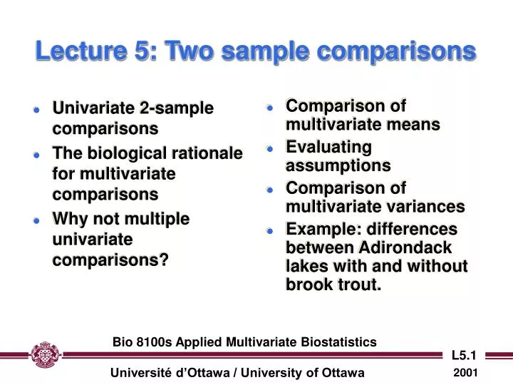
1. Univariate 2-sample comparisons The biological rationale for multivariate comparisons Why not multiple univariate comparisons? Comparison of multivariate means Evaluating assumptions Comparison of multivariate variances Example: differences between Adirondack lakes with and without brook trout. Lecture 5: Two sample comparisons Bio 8100s Applied Multivariate Biostatistics

2. Univariate 2-sample tests s2C • Appropriate when there are two groups to compare (e.g. control and treatment) • In principle, we can compare any sample statistic, e.g., group means, medians, variances, etc. s2T Frequency Control Treatment Bio 8100s Applied Multivariate Biostatistics

3. Control Treatment Two-sample comparisons: control versus experiment • Two plots of corn, one (control) with no treatment, the other (treatment) with nitrogen added • Biological prediction: nitrogen increases crop yield • H0: mT mC (one-tailed) Frequency Yield Bio 8100s Applied Multivariate Biostatistics

4. Control Treatment Comparing means: the t-test • Calculate difference between two means • H0(one-tailed): • Calculate t and associated p Frequency Yield Bio 8100s Applied Multivariate Biostatistics

5. Comparing two means: the multivariate case • Suppose that for each sample unit in two different samples, we measure several variables X1, X2, …XP. • How might we compare the two samples? Bio 8100s Applied Multivariate Biostatistics

6. Possibility 1: multiple univariate tests • In this case, we compare the means of the two samples for each variable individually. • So if we have P variables, we would do Pt-tests (or Mann-Whitney U tests) Bio 8100s Applied Multivariate Biostatistics

7. 1.0 0.8 0.6 Experiment-wise a (ae) 0.4 0.2 0.0 0 2 4 6 8 10 Number of variables Nominal a = .05 Problem 1: controlling experiment-wise a error • For comparisons involving P variables the probability of accepting H0 (no difference) is (1 - a)P. • For 4 independent variables, (1 - a)P = (0.95)4 = .815, so experiment- wise a (ae) = 0.185. • Thus we would expect to reject H0 for at least one variable about 19% of the time, even if the samples differed with respect to none of the four variables. Bio 8100s Applied Multivariate Biostatistics

8. 1.0 0.8 0.6 Experiment-wise a (ae) 0.4 0.2 0.0 0 2 4 6 8 10 Number of treatments Nominal a = .05 Controlling experiment-wise a error at nominal abyadjusting by total number of comparisons • To maintain ae at nominal a, we need to adjust afor each comparison by the total number of comparisons. • In this manner, ae becomes independent of the number of variables… • … but invariably such procedures are too conservative. Bio 8100s Applied Multivariate Biostatistics

9. Controlling ae by adjusting individual a’s Bio 8100s Applied Multivariate Biostatistics

10. Problem 2: reduced power • Samples/groups may differ with respect to their multivariate means but not with respect to the means of any single variable, because of the cumulative effects of several small differences. • Hence, univariate tests will usually have lower power. Sample 2 X2 Sample 1 X1 Bio 8100s Applied Multivariate Biostatistics

11. Problems 3 and 4: loss of information • Univariate tests ignore correlations among variables, which is useful information in itself • With univariate tests, we cannot estimate the extent to which overall differences among samples/groups are due to particular variables. Bio 8100s Applied Multivariate Biostatistics

12. Hotelling’s T2: a multivariate extension of the t-test. • The (2-tailed) null hypothesis is that the vector of means are equal for the 2 populations… • … which implies that the populations are equal on all p variables. Bio 8100s Applied Multivariate Biostatistics

13. Hypothesis testing using Hotelling’s T2. • Conveniently, T2 can be transformed into Fexactly… • … so hypotheses can be tested by comparing observed F to critical values of the F-distribution with p (number of variables) and (n1 + n2 - p - 1) df. Bio 8100s Applied Multivariate Biostatistics

14. Example: body size in Bumpus’s sparrows • H0: mS = mNS (average size of surviving and non-surviving female sparrows is the same) • Variables: total length, alar extent, head length, humerus length, sternum and keel length • H0 accepted. Bio 8100s Applied Multivariate Biostatistics

15. All observations are independent (residuals are uncorrelated) Within each sample (group), variables (residuals) are multivariate normally distributed Each sample (group) has the same covariance matrix (compound symmetry) Assumptions Bio 8100s Applied Multivariate Biostatistics

16. Effect of violation of assumptions Bio 8100s Applied Multivariate Biostatistics

17. Does the experimental design suggest that sampling units may not be independent (e.g. spatiotemporal correlation?) Calculate intraclass R correlation for each variable. Do autocorrelation plots for each variable/group combination to check for serial correlation. Checking independence of observations Bio 8100s Applied Multivariate Biostatistics

18. Checking independence assumption • Run ACFs for all residuals for all groups separately, and check for evidence of autocorrelation among residuals. ACF of residuals of pH for lakes with brook trout Bio 8100s Applied Multivariate Biostatistics

19. Delete observations from each group until independence is achieved (N.B. this will reduce power!) Pool observations into subgroups and use means of subgroups as observations. If non-independence is suspected… Group 1 Group 2 Subgroups Bio 8100s Applied Multivariate Biostatistics

20. Checking multivariate normality • While characterizing MVN is difficult, a necessary (but not sufficient) condition is that each of the variables (residuals) is normally distributed • If there are p variables, there are p sets of estimates and residuals generated for any fitted model. • Check normality by doing normal probability plots for each variable. Normal probability plot of residuals of total length, comparison of survivors and non-survivors from Bumpus data Bio 8100s Applied Multivariate Biostatistics

21. Checking multivariate normality • Calculate percentiles of c2 distribution with p (number of variables) degrees of freedom: • If data are multivariate normal, then for each group, a plot of distances versus percentiles should yield a straight line. • For each group, calculate vector of means and Mahalanobis distance Dj2, j = 1,…, Ni, of each observation from the multivariate mean of group i. • For each group, order distances from smallest to largest: Bio 8100s Applied Multivariate Biostatistics

22. Equality of covariance (C1 = C2) implies that each element of C1 is equal to the corresponding element in C2. This is a very restrictive assumption that is almost never met in practice, so the real question is… …how different are they? Covariance Variance C1 Equality of covariance matrices C2 Bio 8100s Applied Multivariate Biostatistics

23. Checking equality of variances • Plot residuals versus estimates for all variables and check for evidence of heteroscedasticity • Run Levene’s test for heterogeneity of variances for all variables. Residuals versus estimates (total length), comparison of survivors and non-survivors from Bumpus data, Bio 8100s Applied Multivariate Biostatistics

24. Box test for equality of covariance matrices • Calculate ln of the determinant of each group covariance matrix Cicand the pooled covariance matrix C • Use these values to calculate Box’s M • Use k (number of groups) and p (number of variables) to calculate C • For reasonably large Ni (> 20), M(1-C) is approx c2 distributed Bio 8100s Applied Multivariate Biostatistics

25. Box’s test (cont’d) • If the Box test is significant with unequal group sizes, compare determinants of group covariance matrices • If group with smaller N has smaller |C|, test statistics are liberal; if the other way around, they are conservative. • If the Box test is significant with approximately equal group sizes, type I error rate only slightly affected, but power is reduced to some extent Bio 8100s Applied Multivariate Biostatistics

26. Important note! • Box’s test is quite sensitive to deviations from multivariate normality… • … so make sure the MVN assumption is valid before proceeding! Bio 8100s Applied Multivariate Biostatistics

27. Checking assumptions in MANOVA Use group means as unit of analysis Independence (intraclass correlation, ACF) No Yes MVN graph test Ni > 20 Assess MV normality Check group sizes Check univariate normality Ni < 20 Bio 8100s Applied Multivariate Biostatistics

28. Checking assumptions in MANOVA (cont’d) Check homogeneity of covariance matrices MV normal? END Yes Yes Yes No Most variables normal? Groups reasonably large (> 15)? Yes Group sizes more or less equal (R < 1.5)? No Yes Transform offending variables No Transform variables, or adjust a Bio 8100s Applied Multivariate Biostatistics

29. s2C s2T Frequency Control Treatment Comparing two variances: the univariate case • If variances are equal, then s2C = s2T • H0 (Levene’s): • This test is relatively insensitive to non-normality Bio 8100s Applied Multivariate Biostatistics

30. Comparing two multivariate variances I: Levene’s test • Standardize all variables to have zero mean and unit variance. • Calculate absolute value of the difference between the standardized value and the standardized mean (or median) • Compare mean absolute values using Hotelling’s T2. Bio 8100s Applied Multivariate Biostatistics

31. Comparing two multivariate variances II: van Valen’s test • Calculate the difference between the standardized value for each observation and the standardized mean (or median) squared, and sum over variables. • Compare average values for each sample with a univariate t-test (or some such) Bio 8100s Applied Multivariate Biostatistics

32. Example: comparison of Adirondack lakes with and without brook trout • Goal: to elucidate the factors controlling brook trout presence/absence. • Question: do lakes with and without BT differ with respect to certain physiochemical variables, e.g. pH, DO, ANC, elevation, size, etc. BT absent BT present Bio 8100s Applied Multivariate Biostatistics

33. Univariate F Tests Effect SS df MS F P DO 38.330 1 38.330 11.670 0.001 Error 2423.871 738 3.284 PH 47.726 1 47.726 80.256 0.000 Error 438.864 738 0.595 ANC 418836.384 1 418836.384 8.298 0.004 Error 3.72522E+07 738 50477.213 ELEVATION 5192.262 1 5192.262 0.404 0.525 Error 9488005.547 738 12856.376 SA 3731.309 1 3731.309 12.910 0.000 Error 213305.666 738 289.032 Bio 8100s Applied Multivariate Biostatistics

34. Multivariate test-statistics Multivariate Test Statistics Wilks' Lambda = 0.862 F-Statistic = 23.477 df = 5, 734 Prob = 0.000 Pillai Trace = 0.138 F-Statistic = 23.477 df = 5, 734 Prob = 0.000 Hotelling-Lawley Trace = 0.160 F-Statistic = 23.477 df = 5, 734 Prob = 0.000 Bio 8100s Applied Multivariate Biostatistics

35. The conclusion • Lakes with and without brook trout seem to differ with respect to pH, DO, ANC and elevation, but not with respect to elevation • The multivariate means are significantly different, i.e. the null is rejected. • But, before proceeding any further, we MUST check the assumptions of independence, normality, and equality of covariance matrices Bio 8100s Applied Multivariate Biostatistics

36. Checking serial independence using ACF plots • Run MANOVA, save residuals and data • Extract set of residuals for p variables for each group (Brook trout present or absent) • Run ACF on residuals for each variable/group combination. ACF of residuals of pH for lakes with brook trout Bio 8100s Applied Multivariate Biostatistics

37. Checking independence using the intraclass correlation • Get MSs from univariate F tables, and calculate R for each variable • Are the values relatively small? Bio 8100s Applied Multivariate Biostatistics

38. Example: MV normality in Adirondack lakes with brook trout • Run DISCRIM with two groups (BT present and absent), 5 variables (pH, DO, ANC, elevation, SA) to generate Mahalanobis distances • Evidence of non-normality due to skewed distributions of ANC, SA. Bio 8100s Applied Multivariate Biostatistics

39. Box test for equality of covariance matrices • Conclusion: covariance matrices are heterogeneous… • …but analysis based on data which we know do not satisfy normality condition. • So, results are not reliable. • Solution: find transformations such that MVN condition is satisfied, and re-run analyses. Bio 8100s Applied Multivariate Biostatistics