Download
1 / 19
200 likes | 319 Views
Time-dependent modelling of ELMing H-mode at TCV with SOLPS. Barbora Gulejov á, Richard Pitts, Xavier Bonnin, David Coster, Roland Behn, Jan Hor áč ek, Janos Marki OUTLINE. * SOLPS code package * ELM simulation – theory * Simulation of the ELM * Comparison of SOLPS with experiment.

E N D
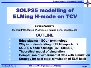
Time-dependent modelling of ELMing H-mode at TCV with SOLPS Barbora Gulejová, Richard Pitts, Xavier Bonnin, David Coster, Roland Behn, Jan Horáček, Janos Marki OUTLINE • * SOLPS code package • * ELM simulation – theory • * Simulation of the ELM • * Comparison of SOLPS with experiment
Scrape-Off Layer Plasma Simulation Suite of codes to simulate transport in edge plasma of tokamaks B2 - solves 2D multi-species fluid equations on a grid given from magnetic equilibrium EIRENE - kinetic transport code for neutrals based on Monte - Carlo algorithm SOLPS 5 – coupled EIRENE + B2.5 Mesh plasma background => recycling fluxes 72 grid cells poloidally along separatrix 24 cells radially B2 EIRENE Sources and sinks due to neutrals and molecules measured Main inputs: magnetic equilibrium Psol = Pheat – Pradcore upstream separatrix density ne Free parameters: cross-field transport coefficients (D┴, ┴, v┴) systematically adjusted
Edge localised mode (ELM) H-mode Edge MHD instabilities Periodic bursts of particles and energy into the SOL - leaves edge pedestal region in the form of a helical filamentary structure localised in the outboard midplane region of the poloidal cross-section Dα divertor targets and main walls erosion first wall power deposition ELMing H-mode=baseline ITER scenario Energy stored in ELMs: TCV 500 J JET 200kJ ITER 8-14 MJ => unacceptable => LFS HFS W~600J Small ELMs on TCV – same phenomena ! => Used to study SOL transport
Type III Elming H-mode at TCV Ip = 430 kA, ne = 6 x 10¹⁹ m-3 , felm = 230 Hz # 26730 ELMs - too rapid (frequency ~ 200 Hz) for comparison on an individual ELM basis => Many similar events are coherently averaged inside the interval with reasonably periodic elms telm ~ 100 μs tpost ~ 1 ms tpre ~ 2 ms Pre-ELM phase = steady state ELM = particles and heat are thrown into SOL ( elevated cross-field transport coefficients) Post-ELM phase
Simulation of pre-ELM = steady state of H-mode presented at PSI 17, Hefei,China and published in JNM May 2006 D┴,Χ┴= radially constant in divertor legs upstream targets inner outer Jsat [A.m-2] LP, average SOLPS D┴= 3 m2.s-1 in div.legs 1m2.s-1 in SOL Χ┴= 5 m2.s-1 in div.legs 6 m2.s-1 in SOL NO DRIFTS here But simulations with DRIFTs show early promise of expected effects Te [eV] * * ne [m-3] Very good overall match Ansatz D[m2.s-1] Χ[m2.s-1] r-rsep r-rsep Perp.heat flux[MW.m-2] LP, average SOLPS Good basis for time-dependent ELM simulation <=> Pre-ELM must be time-dependent too! + equal time-steps for kinetic and fluid parts of code ~ 10-6s v[m.s-1] inner same solps result! Vperp=0 * IR outer * r-rsep
Simulation of ELM * Instantaneous increase of the cross-field transport parameters D┴, ┴, v┴! 1.) for ELM time – from experiment coh.averaged ELM = tELM = 10-4s 2.) at poloidal location -> expelled from area AELM at LFS From the cross-field radial transport can be estimated the combination of transport parameters corresponding to the given expelled energy WELM, tELM and AELM Dα Many different approaches possible => changes in D┴, ┴only or in v┴too … W~600J time AELM= 1.5m2 W = 600 J * D┴ Diff.[eV.m-2.s-1] D┴ Conv.[eV.m-2.s-1] ┴
Tools to simulate ELM in SOLPS Several options in SOLPS transport inputfiles : *Multiplying of the transport coefficients in the specified poloidal region * In 3 different radial regions (core, pedestal, SOL) by different multipliers Added new options: *Poloidal variation of the multiplicator * Step function * Gaussian function * Choosing completely different shape of radial profile for chosen poloidal region main SOL ELM Inner div.leg main SOL No TB ELM x M preelm outer div.leg core pedestal wall
Experimental data to constrain the code: * Energy expelled by the ELM through separatrix (DML) ~ 600 J * Time of ELM-rise (D coavelm) ~ 100 μs * Jsat at the targets * Heat flux at outer target (IR soon) * Upstream ne,Te (TS) -> just orientation Simulation of ELM
Simulation of ELM - results Upstream profiles D,Chi (ELM): Same shape as preELM => TB, Just multiplied D x 100, Chi x 8 D,Chi (ELM): smaller TB + Gaussian function poloidally D, Chi increased only locally ! ne [m-3] ne [m-3] Te [eV] Te [eV] r-rsep r-rsep
Comparison with TS – R.Behn Time evolution of D┴ and ne no TB TB D┴ ne time tELM=100 µs ne TS measurements (R.Behn) => *Drop in pedestal width and height appears only for ne SOLPS*bigger pedestal collaps * higher ne and Te in SOL But the right tendency – pedestal collapse time + different ELMing H-mode shots ! R-Rsep no TB TB Te [eV] R-Rsep
Simulation of ELM - results Target profiles D,Chi (ELM): smaller TB + Gaussian function poloidally D,Chi (ELM): Same shape as preELM => TB, Just multiplied D x 100, Chi x 8 targets targets “removal” of TB => higher values at the targets outer outer inner inner Jsat [A.m-2] SOLPS Jsat [A.m-2] SOLPS 30 27 preELM ELM 22 16 LP coav data preELM ELM 40 inner Te [eV] Te [eV] Jsat [A.m-2] preELM ELM outer ne [m-3] 35 ne [m-3] Jsat [A.m-2]
Target profiles – Heat fluxes Simulation of ELM - results D,Chi (ELM) :Same shape as preELM => TB, just multiplied D x 100, Chi x 8 D,Chi (ELM): smaller TB + Gaussian function poloidally Like Jsat, Te, and ne, heat flux is higher for the case with smaller TB inner inner IR data available soon (J. Marki) 16 outer 20 outer Time-dep. heat flux estimated from LP measurements at outer target 9 R.Pitts, Nuc.Fusion 2003
ELM-Time evolution of jsat at targets outer target ELM LP 5 pre-ELM ELM post-ELM SOLPS Dα post-ELM pre-ELM Jsat [A.m-2] LP 20 SOLPS Inner R.Pitts, Nuc.Fusion 2003
ELM-Time-dependent solution at targets targets TB during ELM midplane separatrix TB during ELM inner outer ELM Jsat [A.m-2] Jsat [A.m-2] ne [m-3] ne [m-3] Te [eV] Te [eV] Ti [eV] time [s] time [s] Ti [eV] Density is fixed at midplane separatrix => can’t change too much at the targets either => Jsat can increase mostly through Te,Ti => Necessary to increase D more then Chi in order to act on increase of ne time [s]
ELM-time-evolution of jsat at targets targets outer inner Jsat [A.m-2] Jsat [A.m-2] ELM rise time LP 20 LP 5 Compared with LP close to strike point => Not exactly the same position SOLPS SOLPS time [s] time [s]
Timedependence of target Te,Ti SOLPS inner outer Te is rising quicker then Ti Te [eV] Te [eV] Propagation down to the target from upstream pedestal Ti [eV] Ti [eV] Timedependence of simulated Te,Ti (D.Tskhakaya) for 120kJ ELM at JET (sheat heat coeff assumed 8) R.Pittts, IAEA,2006
Timedependence of target Te,Ti ELM ‘end’ SOLPS ELM ‘end’ outer inner peak Te [eV] peak Ions are arriving to target later then electrons (~16 μs) In reality should be more, but : 1.) probably more collisional 2.) SOLPS – equipartition of energy between ions and electrons => reasonable shift of Te,Ti peaks Ti [eV] R.Pittts, IAEA,2006