Download
1 / 31
320 likes | 509 Views
Sanjib Sharma Joss Bland-Hawthorn (University of Sydney, Australia) RAVE collaboration. Kinematic Modelling of the Milky Way using RAVE and GCS. http://physics.usyd.edu.au/~sanjib/rave_sharma.pdf. How was Milky Way formed?. Stars formed. J f. J i. DM. Chemical enrichment. Gas.

E N D
Sanjib Sharma Joss Bland-Hawthorn (University of Sydney, Australia) RAVE collaboration Kinematic Modelling of the Milky Way using RAVE and GCS. http://physics.usyd.edu.au/~sanjib/rave_sharma.pdf
How was Milky Way formed? Stars formed Jf Ji DM Chemical enrichment Gas Gas Accretion Secular heating, non circular orbits
Basic model of the Milky Way • fC(r,v,t,m,Z) • Thin disc, Thick Disc, Stellar Halo, Bar-Bulge. • f(r,v,t,m,Z) ∝ p(r,t) p(m|t) p(Z|t) p(v|r,t) • position-age mass FeH velocity
Basic model of the Milky Way • fC(r,v,t,m,Z) • Thin disc, Thick Disc, Stellar Halo, Bar-Bulge. • f(r,v,t,m,Z) ∝ p(r,t) p(m|t) p(Z|t) p(v|r,t) • position-age mass FeH velocity • The Besancon model (BGM). • p(r,t) p(m|t) p(Z|t) the main assumption • Padova Isochrones
The kinematic model: Gaussian distribution function Age Velocity dispersion (AVR) Asymmetric Drift
The kinematic model: Gaussian distribution function Age Velocity dispersion (AVR) Asymmetric Drift
The kinematic model: Gaussian distribution function Age Velocity dispersion (AVR) Asymmetric Drift
The kinematic model: Gaussian distribution function Age Velocity dispersion (AVR) Asymmetric Drift
Cause of Asymmetric drift • Vφ is shifted and has asymmetric distribution • Cause of asymmetric drift • More stars with small L (exponential disc) • Stars with small L are hotter (larger σ) so more likely on elliptical orbits. • In elliptical orbit most time spent at apogee so at large R>Rc. Sun
The kinematic model: The Shu distribution function • L is angular momentum, • ER=E-Ec(L)is the energy in excess of that required for circular motion with a givenL. • Naturally handles asymmetric distribution. • Note vertical and planar motion are decoupled, potential separable in Φ(R,z)=Φ(R)+Φ(z).
Circular velocity profile • The circular velocity can have both radial and vertical dependence. • vc(R,z)=[v0+αR(R-R☉ )] [ 1/(1+αz(z/kpc)1.34) ] • Two popular models of Milky Way's 3D potential DB98 and LM10 shown below, have αz ~ 0.0374 • In reality vertical motion is coupled to planar motion, so asymmetric drift also has a dependence on z. We incorporate it into αz. We expect αz > 0.0374
Model parameters explored θ={Set of parameters}
Kinematic analysis using RAVE and GCS • GCS: A color magnitude limited sample of stars with (x,v). Very local 120 pc. (about 5000 stars) • RAVE a spectroscopic survey of about 500,000 stars with accurate, (l,b,vlos). 1- 2kpc
RAVE analysis • No use of proper motion or distances • No use of J-K, Teff, log g p(θ | l,b,vlos) ~ p(l,b,vlos | θ ) p(θ)
Questions? • Is the Gaussian model correct? • What are the correlations between different parameters? • Does GCS and RAVE give similar values? • What are U☉,V☉,W☉, vc(R☉)? • Schonrich et al (2010) (11.1, 12.24, 7.25) km/s, 220+- 30 km/s W V Sun U Galactic Center
Proper motion of Sgr A* • vc , V☉andR☉are difficult to measure but • Sgr A* at the center of galaxy, 8 yr baseline • Ω☉=(vc+V☉ )/R☉ ~30.24 km/s/kpc (Reid & Brunthaler 2004). • For R☉=8.0 kpc, (vc+V☉)~242 km/s • Recently Bovy using APOGEE data find, • vc=218(+- 6) km/s, V☉ = 26(+- 3) km/s, • Rσthin negative. • Since local V☉ ~ 10 km/s, LSR might be on a non circular orbit.
Method of fitting analytical models to data • Bayesian data analysis. We use MCMC to explore the full posterior distribution of model parameters. • p(θ | l,b,vlos) ~ p(l,b,vlos | θ ) p(θ) • Data is color magnitude limited sample of stars with (l,b,vlos). • So we have to marginalise over • (t 'Age',m 'mass', Z '[Fe/H]') • and also (d, vl, vb). • p(l,b,d,t|S) = ∬ p(l,b,d,t,m,Z) S(l,b,t,m,Z) dm dZ • p(l,b,d,t,m,Z) comes from the Besancon Galaxy model. • S(l,b,t,m,Z) is the selection function unique to each survey • Computation done numerically using the code GALAXIA
Method of fitting analytical models to data • Full exploration of parameter space using MCMC is computationally costly. In RAVE we have more than 200,000 stars which makes the task even more challenging. • Instead of doing integrals • We set up the problem as a hierarchical Bayesian model. • Metropolis-Within-Gibbs was found to be useful.
Problems with Gaussian models • In Gaussian models Rσthinis strongly correlated with V☉. • Moreover, for RAVE dataRσthinis negative while for GCS data it is positive. • So the Gaussian model gives inconsistent results when applied to RAVE and GCS data sets.
RAVE-GAUSS • Marginalised posterior distribution of model parameters. • The anti-correlation of Rσthin and V☉ sun can be seen • V☉ and vcaffected by αz
RAVE-SHU In the Shu model the azimuthal motion is coupled to radial motion so it has 3 fewer parameters. This helps to resolve the Rσthin – V☉degeneracy.
Best fit Gaussian vs Shu models • The Gaussian model fails to properly fit the wings of the distribution. • The reason that the Gaussian model gives inconsistent results for RAVE and GCS is because it is not a good description of the data.
Best fit parameters for the Shu model αz free makes vc go up. 232.8+7.53=240.33 km/s. GCS and RAVE also match, σR similar for thin and thick Quantities in magenta were kept fixed during fitting. Units are in km/s and kpc
Rave velocity distribution compared to models. • The Shu model fits the RAVE data well.
How well does the RAVE best fit model fit the GCS data? • The Shu-RAVE slightly overestimates the right wing of the V distribution. • The discrepancy is probably due to significant amount of substructure in the GCS data which can potentially bias the GCS best fit model.
Systematics • Dependence on gradient dvc/dR • Rsun dependence • Isochrone magnitudes • p(r,t) the BGM model.
Systematics • Kinematic models are not fully self-consistent • The vertical dependence handled by a fudge factor. • Dynamically self-consistent models based on action integrals.
Conclusions • Using only (l,b,vlos) data from RAVE survey we obtain • good constraints on a number of kinematic parameters of the Milky Way. • Deficiency of a Gaussian model is clearly exposed by RAVE data • (high V☉,negative Rσthin) • Vc, V; ; • model dependent • Neglecting vertical dependence of kinematics can lead to undestimation of Vc. • We find vcirc~232 km/s and V☉ ~7.54 km/s, which gives Ω☉=(vc+V☉ )/R☉ ~ 30.04 km/s/kpc • in good agreement with Sgr A* proper motion of 30.24 km/s/kpc (Reid & Brunthaler 2004). • The best fit RAVE model also fits the GCS data well. • GCS V☉is lower by 2 km/s. • In future, fitting a dynamical model that takes into account both the spatial and kinematic components together should lead to more robust analysis.
Publicly available codes that might be of interest to you GALAXIA- http://galaxia.sourceforge.net • A general purpose binary file format publicly available at • Automatic endian conversion, data type conversion • Store multiple data items in same file • Time to locate an item, almost independent of number of items. Due to use of inbuilt hashtable • Support for homogeneous multidimensional arrays and structures (also nested structures) • Not tied to one programming languange. • API available in IDL, MATLAB, Python,C,C++, Fortran, Java Galaxia is a code for generating a synthetic model of the galaxy. The input model can be analytical or one obtained from N-body simulations. The code outputs a catalog of stars according to user specified color magnitude limits. EBF-http://ebfformat.sourceforge.netEfficient Binary data Format“Put fun back into numerical computing, Use EBF”
Comparison with Besancon 43.1 27.8 17.5