Download
1 / 18
180 likes | 329 Views
Geodetic Reference Frames In Presence of Crustal Deformations. Martin Lidberg 1,2 , Maaria Nordman 3 , Jan M. Johansson 1,4 , Glenn A Milne5, Hans-Georg Scherneck 1 , Jim L Davis 6 1 Onsala Space Observatory, Chalmers, Sweden 2 Lantmäteriet (National Land Survey of Sweden)

E N D
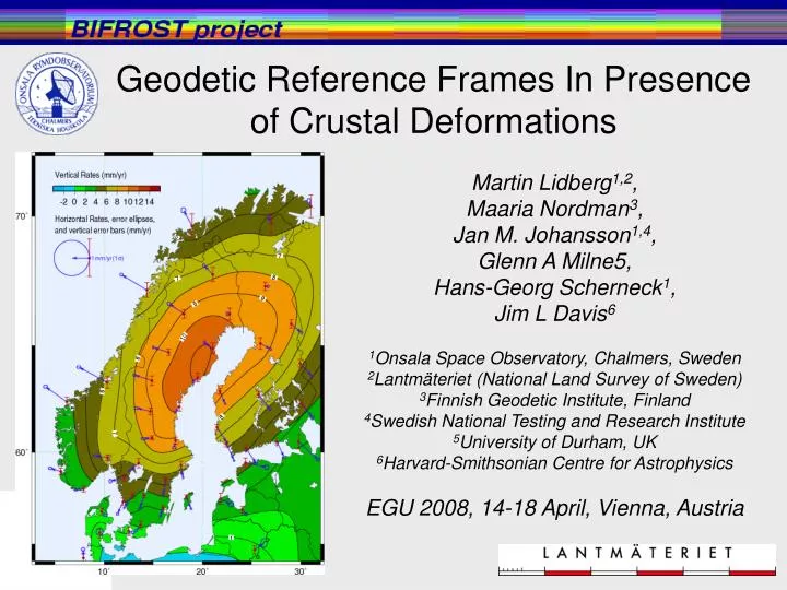
Geodetic Reference Frames In Presence of Crustal Deformations Martin Lidberg1,2, Maaria Nordman3, Jan M. Johansson1,4, Glenn A Milne5, Hans-Georg Scherneck1, Jim L Davis6 1Onsala Space Observatory, Chalmers, Sweden 2Lantmäteriet (National Land Survey of Sweden) 3Finnish Geodetic Institute, Finland 4Swedish National Testing and Research Institute 5University of Durham, UK 6Harvard-Smithsonian Centre for Astrophysics EGU 2008, 14-18 April, Vienna, Austria
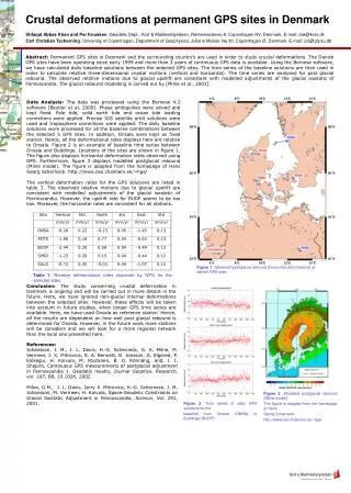
Effects of the land uplift • First determination of the land uplift related to sea level • apparent • land uplift • Determination of horizontal rates and absolute land uplift values; • the purpose of BIFROST
Outline • The BIFROST GPS network • GPS analysis • Reference frame realization • Time series analysis and data editing • Evaluation of the velocity field • Address noticed problems and possible causes • Conclusions
The extended BIFROST network • The analysis includes: • Public sites from IGS and EPN (EUREF Permanent Network) (blue dots ) • Sites not in the public domain (yellow diamonds ) • Totally: 83 sites • Period of analysis: • Aug. 1993 – Oct. 2006
GAMIT / GLOBK GAMIT (GPS analysis) Traditional analysis strategy 10° elevation cut off angle Trop. zenith delay & gradients the Niell 1996 mapping functions Relative antenna PCV values (“absolute” PCV not used so far) a priori orbits from SCRIPPS GLOBK (combination & ref. frame) combination of sub-networks reference frame realization. Combine the regional analysis with “complete IGS analysis” from SCRIPPS (GAMIT h-files). Satellite orbits are given loose constraints in the quasi-observations. GPS analysis strategy GIPSY • Precise Point Positioning (PPP) using JPL products • And ambiguity fixing • Used to validate the GAMIT/GLOBK solution
Combination for “global solution” & reference frame realization ITRF2000: 43 “good” sites as candidates for the daily stabilization. in GLOBK. ITRF2005: 78 sites as candidates. - Include breaks from ITRF2005 coordinate list
(ITRF2000)Results from stabilization (ITRF2005) Scale (ppb) postfit RMS (mm) No used sites
Example of time series of GPS positions • De-trended position time series from Vilhelmina (64°N) for the complete period • Aug. 1993 – Oct 2006 • 1993-1996: • - some “bad” antenna radoms • PROBLEMS !!!??? • Non-linear time-series in the vertical: • Bent “banana”-shape ??? • - Or rate change by 2003 ??? • Tide model problem?? • Watson, Tregoning, Coleman (2006) “Impact of solid earth tide models on GPS coord. and trop. time series”, GRL.
New combination - with my own global analysis • The global network: • 35 selected sites. (black squares ) • - Cover the globe - Connect regional & global analysis • - Include “good” sites for reference frame realization • Reference frame sites: • 23 sites as candidates (yellow circles )
Combined Regional BIFROST + “35-site” global - Vertical “banana-shape” heavily reduced!!! (maybe not eliminated..) - In the analysis we have “stable” sites with +10 yr observations, and “new” sites (< 5 yr). Two step reference frame approach 1. Determine pos+vel for 27 “good sites” (Swe+Fin+some EPN) from “stable” period 1998 to 2004 (7yr). 2. Apply 6-par transf. (no scale) of all daily solutions to the “regional” frame defined above.
Derived velocity field relative to Eurasia Red: ITRF2000 (eura) Green: ITRF2005 (eura) ITRF2000: removed the Eurasia plate tectonic motion using the ITRF2000 Euler pole for Europe ITRF2005: transformed (rotated) to the ITRF2000_eura velocities RMS of velocity at 7 European IGS sites: 0.5 mm/yr level -> suggest a successful reference frame realization. For POTS and METS; “my” velocities and official ITRF2005 agree by: North: 0.2 mm/yr East: 0.3 mm/yr Up: 0.3 mm/yr
Glacial Isostatic Adjustment (GIA) Glaciations cause change of load from ice and ocean to the earth. This load cause deformation of the earth shape and mass re-distribution. Updated GIA model (Milne et al 2001) Ice history model from Lambeck 120 km lithosphere, upper mantle visc. 51020 Pas lower mantle visc. 51021 Pas Thanks Glenn Milne, Maaria Nordman, Pippa Whitehouse!!
Vertical velocity • ITRF2005 • ITRF2000 • GIA model • Ekman (1998) based on: • mareographs and levellings, • 1.2 mm/yr eustatic sea level rise • change of the geoid based on Ekman & Mäkinen (1998) • Compared to the ITRF2000 • values: • mean Std (mm/yr) • ITRF2005 0.4 0.1 • GIA model -0.4 0.5 • Ekman -0.4 0.6
The new station velocities Validation using GIPSY (0.1, 0.1, 0.2) (n,e,u) mm/yr New GIA model minus GPS, “best sites” (0.3, 0.2, 0.3) (n,e,u) mm/yr The new GAMIT/GLOBK solution (in ITRF2005) And GIA model
The “hole” in the sky plot at high latitude sites! • Satellite geometry at two locations • Will this cause error in height, if e.g. elevation dependence (antenna models) and mapping functions are imperfect?
Vilhelmina, 64°N BIFROST+ global SOPAC IERS1996 tide model Relative antenna models BIFROST+ Own global 35 site net Mixed IERS1996+ IERS2003 tide model Relative antenna models 45 global+35 EPN sites IERS2003 tide model Absolute antenna models GMF mapping function (Only every 10 day)
Conclusion and outlook GPS-velocities and GIA-model agree at - 0.4 mm/yr level (1) horizontal - 0.5 mm/yr level (1) vertically GIA model explain observed velocities to 0.5 mm/yr!! OK for coordinate transformation and “geo-referencing” purposes;but for sea level work (exploring GPS and Tide gauge obs.) we must be careful and continue the work regarding: • “long term stability in GNSS results” • improvements in the reference frame! in order to reached the 0.1 mm/yr goal! Proper velocity estimation need correct models in the GPS analysis! • Therefore the re-processing of IGS, with “best” models is very important (abs. antenna models, tide model, mapping function, ionosphere..) • Will be a base for the next improved ITRF200x!