Download
1 / 30
300 likes | 391 Views
L’histoire de la formation stellaire dans l’univers avec les ELT et ALMA. Un exemple de distribution spectrale d’énergie GALEX-ELAIS-SWIRE nécessité de coupler UV-optique et FIR-submm. La contribution de l’émission des poussières cro ît avec z. Z= 0 , 0.3 , 0.5 , 0.7 & 1.0

E N D
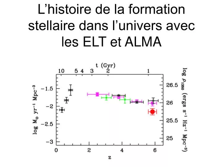
L’histoire de la formation stellaire dans l’univers avec les ELT et ALMA
Un exemple de distribution spectrale d’énergie GALEX-ELAIS-SWIREnécessité de coupler UV-optique et FIR-submm
La contribution de l’émission des poussières croît avec z • Z= 0, 0.3, 0.5, 0.7 & 1.0 • Plus grande evolution en FIR qu’en UV • mais forte évolution des galaxies de faible luminosité en UV
Comment mesurer le SFR en UV-optique? continuum UV ou raies d’émission
Mesure du continuum: Pour détecter des galaxies à z=7 avec L=L* etmAB= 28.7 0.01 < L/L* < 0.1 et 31.2 < mAB < 33.7
ALMA: Un exemple de détection a haut redshift M82 from ISO, Beelen and Cox, in preparation • As galaxies get redshifted into the ALMA bands, dimming due to distance is offset by the brighter part of the spectrum being redshifted in. Hence, galaxies remain at relatively similar brightness out to high distances.
ALMA Deep FieldPoor in Nearby Galaxies, Rich in Distant Galaxies Source: Wootten and Gallimore, NRAO Nearby galaxies in ALMA Deep Field Distant galaxies in ALMA Deep Field
Hubble Deep FieldRich in Nearby Galaxies, Poor in Distant Galaxies Source: K. Lanzetta, SUNY-SB Nearby galaxies in HDF Distant galaxies in HDF
ALMA Redshift Survey 4’×4’ Field Step 1 A continuum survey at 300 GHz, down to 0.1 mJy (5σ). This requires 140 pointings, each with 30 minutes of observation, for a total of 3 days. Such a survey should find about 100-300 sources, of which 30-100 sources will be brighter than 0.4 mJy. This field is twice the size of the HDF. Image 3000x3000 pixels x 1024 frequencies. Step 2 A continuum and line survey in the 3 mm band down to a sensitivity of 7.5 mJy (at 5σ). This requires 16 pointings, each with 12 hours of observation, so a total of 8 days. The survey is done with 4 tunings covering the 84-116 GHz frequency range. Image 1000 x 1000 pixels x 4096 frequencies. The 300 to 100 GHz flux density ratio gives the photometric redshift distribution for redshifts z > 3-4. For expected line widths of 300 km/s, the line sensitivity of this survey is 0.02 Jy.km/s at 5σ. Using the typical SED presented earlier this should detect CO lines in all sources detected in Step 1. At least one CO line would be detected for all sources above z = 2, and two for all sources above z = 6. The only ``blind'' redshift regions are 0.4-1.0 and 1.7-2.0. Step 3 A continuum and line survey in the 210-274 GHz band down to a sensitivity of 50 mJy (at 5σ). 8 adjacent frequency tunings would be required. On average, 90 pointings would be required, each with 1.5 hours, giving a total of 6 days. Together with Step 2, this would allow detection of at least one CO line for all redshifts, and two lines for redshifts greater than 2. 2000x2000 pixels by 8192 frequencies. N.B.Three ‘data products’ of substantial complexity to assimilate.
Comparaison avec une galaxie plus « normale »NGC 4414(J. Braine) 0.1 mJy ne sera peut-être pas une limite assez profonde Le champ d’ALMA n’est pas très favorable aux surveys
Un instrument submm (type SCUBA) sur les ELT serait plus efficace pour un survey (projet SCELT-SCOWL)
SCOWL sur OWL et ALMA : quelques comparaisons préliminaires SCOWL ALMA • Matrice 20000 pixels de 1 arcsec2 • 0.17 mJy en 1h à 10 @ 350 m • Survey grande surface • 1 deg2, 5 = 0.1 mJy • 39 nuits (1nuit = 12h) • Survey profond • 10 arcmin2, 5 = 0.02 mJy • 3 nuits
En résumé: • La mesure statistique de l’histoire de la formation stellaire nécessite des grands champs et peu de résolution spectrale • ELT: SFR jusqu’à z 5-7 puis compétition avec JWST. ELT meilleur en NIR, couvre le visible • ALMA: petit champ, difficile de faire de grands surveys, FIR-submm sur un ELT plus adapté • ELT vis-NIR et ALMA très adaptés aux études détaillées et physiques cf. présentations de M. Gérin et F. Hammer
Un instrument submm sur un ELT sera plus efficace qu’ALMA pour des grands relevés
SPICAThe Cosmic Star Formation Density : Building a Sample of 0.5 ≤ z < 3.0 Lyman Break & Star-Forming Galaxies to compute Total Star Formation Rates Véronique Buat & Denis Burgarella Obs. Astronomique Marseille Provence LAM
General Objectives Multi- data @ low-to-moderate R to study galaxies and their properties (z) : • Dust Content • Star Formation (rate, density)
R = 40 20 13 10 Detection Limit 5, 1h (Jy) Wavelength (m) Instrumental Assumptions • Detection limit over the band 50 - 200 m is taken • to ~ 50 Jy in 1h and at 5 (04-2005) )= 5 cm-1
Confusion effects • Several confusions : • Cirrus emission • Extragalactic sources • Latter will be dominant for large telescopes like Herschel and SPICA (Kiss, Klass & Lemke 2005 A&A 430, 343) • Dole et al. (2004 ApJS 154, 93) compute total confusion limits ( ) for SPICA
Back to the original paper by Helou & Breichman (1990, In ESA, From Ground-Based to Space-Borne Sub-mm Astronomy p. 117) (1) • Decomposition of confusion limit into several components: • Telescope & Detector • Bright cirrus • Galaxies • (1) valid for a 4-m passively cooled telescope in Earth orbit (not SPICA) (2) (3)
LBGs (30Msun/yr) > 2 not detected in 1h ( )but detected in 100h ( ) and even at z = 3 for SFRIR > 30Msun/yr ( ) ALMA ALMA Takeuchi et al. (2005)
Proposition of Program for SPICA/ESI • Title: Evaluating the Total (UV + FIR) Star Formation Density • Field of view : as large as possible but about 2’ x 2’ seems reasonable • Wavelength range : 40 to 100 m • Spectral resolution : 10 to 50 • Spatial resolution : diffraction limited • Need for SPICA : no existing facility can observe in the FIR down to ~ 10 Msun / yr over a large field of view