Download
1 / 14
140 likes | 221 Views
Waveform Consistency Test in Burst Detection. Laura Cadonati LSC meeting, Hannover August 20, 2003. Test goal. The LIGO Burst Search pipeline uses Event Trigger Generators (ETGs) to flag times when “something anomalous” occurs in the strain time series

E N D
Waveform Consistency Test in Burst Detection Laura Cadonati LSC meeting, Hannover August 20, 2003
Test goal The LIGO Burst Search pipeline uses Event Trigger Generators (ETGs) to flag times when “something anomalous” occurs in the strain time series burst candidate events (Dt, Df, SNR) Events from the three LIGO interferometers are brought together in coincidence (time, frequency, power). In order to use the full power of a coincident analysis: • Are the waveforms consistent? To what confidence? • Can we suppress the false rate in order to lower thresholds and dig deeper into the noise? Cross correlation of coincident events Hannover LSC meeting, August 20, 2003
Data Conditioning • Decimate and high-pass few seconds of data around event 100-2048 Hz • Remove predictable content (effective whitening/line removal): train a linear predictor error filter over 1 s of data (1 s before event start), • apply as second order sections model using zero-phase filtering - described in S. Chatterji’s talk on data conditioning (LIGO-G030439) • emphasis on transients, avoid non-stationary, correlated lines. H1 L1 Hannover LSC meeting, August 20, 2003
r-statistic Linear correlation coefficient or normalized cross correlation for the two series {xi} and {yi} • NULL HYPOTHESIS: the two (finite) series {xi} and {yi} are uncorrelated • Their linear correlation coefficient (Pearson’s r) is normally distributed around zero, with s = 1/sqrt(N) where N is the number of points in the series (N >> 1) S = erfc (|r| sqrt(N/2) ) double-sided significance of the null hypothesis i.e.: probability that |r| is larger than what measured, if {xi} and {yi} are uncorrelated C = - log10(S) confidence that the null hypothesis is FALSE that the two series are correlated Hannover LSC meeting, August 20, 2003
What delay? Shift {yi} vs {xi} and calculate: rk ; Sk ; Ck …then look for the maximum confidence CM Time shift for CM = delay between IFOs Shift limits: ±10 ms (LLO-LHO light travel time) Integration time t: • If too small, we lose waveform information and the test becomes less reliable • If too large, we wash out the waveform in the cross-correlation • Test different t’s and do an OR of the results (20ms, 50ms, 100ms) How long? Delay and Integration Time Hannover LSC meeting, August 20, 2003
Noise only (no added signal) r-statistic vs lag KS stat = 9.9% significance=37.6% KS passed Simulated Sine-Gaussian Q=9, f0=554Hz (passed through IFO response function) hpeak=1e-18 [strain]; hrss=5e-20 [strain/rtHz] r-statistic vs lag L1 • L1-H1 pre-processed waveforms and r-statistic plot • integration time t = 20 ms, • centered on the signal peak time. • a Kolmogorov-Smirnov (KS) test states the {rk}distribution is NOT consistent with the null hypothesis. • there is less than 0.1% probability that this distribution is due to uncorrelated series. • On to the calculation of the confidence series and of its maximum CM (j) lag [ms] time [ms] Kolmogorov-Smirnov test H1 measured CDF Null hypothesis CDF KS stat = 44.3% significance<0.1% KS fails - keep this event abs(r-statistic) time [ms] confidence vs lag Max confidence: CM(t0) = 13.2 at t2 -t1= - 0.7 ms Hannover LSC meeting, August 20, 2003 lag [ms]
Simulated Sine-Gaussian Q=9, f0=361Hz (passed through IFO response function) hpeak=1e-18 Simulated 1 ms Gaussian (passed through IFO response function) hpeak=1e-18 r-statistic vs lag r-statistic vs lag L1 L1 lag [ms] time [ms] time [ms] lag [ms] H1 H1 KS stat = 68.4% significance<0.1% KS fails KS stat = 41.2% significance<0.1% KS fails time [ms] abs(r-statistic) abs(r-statistic) time [ms] Max confidence: CM(t0) = 10.7 at t2 -t1= 0 ms Max confidence: CM(t0) = 16.6 at t2 -t1= 2.9 ms confidence vs lag confidence vs lag Hannover LSC meeting, August 20, 2003 lag [ms] lag [ms]
Hardware injection Sine-Gaussian Q=9, f0=554Hz - April 9 2003 hpeak~1e-18 hpeak~6e-21 [strain/rtHz] r-statistic vs lag r-statistic vs lag L1 L1 lag [ms] time [ms] time [ms] lag [ms] H1 H1 KS stat = 32% significance<0.1% KS fails KS stat = 19.5% significance=0.3% KS fails time [ms] abs(r-statistic) time [ms] abs(r-statistic) Max confidence: CM(t0) = 4.1 at t2 -t1= -0.9 ms confidence vs lag Max confidence: CM(t0) = 4.2 at t2 -t1= 2.9 ms confidence vs lag Hannover LSC meeting, August 20, 2003 lag [ms] lag [ms]
Dt = - 10 ms Dt = + 10 ms Scanning the Trigger Duration DT • Partition trigger in Nsub=(2DT/t)+1 subsets and calculate CM (j) (j=1.. Nsub) • Use Gab = maxj(CM(j)) as the correlation confidence for a pair of detectors over the whole event duration Hannover LSC meeting, August 20, 2003
CM(j) plots G12 =max(CM12) • Each point: max confidence CM(j) for an interval twide(here: t = 20ms) • Define a cut (pattern recognition?): • 2 IFOs: • G=maxj(CM(j) ) > b2 • 3 IFOs: • G=maxj(CM12+ CM13+ CM31)/3 > b3 • In general, we can have b2 b3 • b=3: 99.9% correlation probability G13 =max(CM13) G23 =max(CM23) G=max(CM12 +CM13+CM23)/3 Hannover LSC meeting, August 20, 2003
Open Issues • Calibration • Needed to account for waveform distortions due to frequency-dep calibration • Time resolution • Depends on waveform • Affected by detector response function • Implement phase calibration to match IFOs? • Affected by pre-processing filters • Do a second test pass with less aggressive filters? • At the moment, no use is made of the delay time in assessing the confidence • Implement a T-statistic test? Hannover LSC meeting, August 20, 2003
Triple-coincidence efficiency for 1 ms gaussians • Same amplitude event injected in L1, H1, H2 • 0.2 sec around the injection time passed through the r-test. • Sigmoid fit to efficiency curve: 50% at hpeak=2e-19 S1 TFCLUSTERS 9.5e-18 R-statistic 1.9e-19 Old TFCLUSTERS 1.5e-18 Old POWER 4.7e-19 Hannover LSC meeting, August 20, 2003
Triple-coincidence efficiency for 554 Hz Q=9 sine gaussians • Same amplitude event injected in L1, H1, H2 • 0.2 sec around the injection time passed through the r-test. • Sigmoid fit to efficiency curve: 50% at hpeak=1.2e-19 hrss=6e-21 strain/rtHz S1 TFCLUSTERS 2.7e-18 R-statistic 1.2e-19 Old TFCLUSTERS 6e-19 Old POWER 2.7e-19 Hannover LSC meeting, August 20, 2003
Triple-coincidence efficiency for 361 Hz Q=9 sine gaussians • Same amplitude event injected in L1, H1, H2 • 0.2 sec around the injection time passed through the r-test. • Sigmoid fit to efficiency curve: 50% at hpeak=6e-20 hrss=3.6e-21 strain/rtHz R-statistic 6e-20 S1 TFCLUSTERS 2e-18 Old TFCLUSTERS 3e-19 Old POWER 1.4e-19 Hannover LSC meeting, August 20, 2003